

Matchup Probabilities in Major League Baseball
This article was written by Matt Haechral
This article was published in Fall 2014 Baseball Research Journal
Predicting the results of matchups in baseball, or any sport for that matter, is compelling not only for the ability to possess seemingly prognosticative powers, but also for its applications in simulated games and evaluating players. In his 1981 Baseball Abstract, statistician and sabermetrics pioneer Bill James, in collaboration with Dallas Adams, introduced a formula for predicting the winner of a matchup between two teams. His formula for estimating the probability that team X beats team Y, which James referred to as the log5 method, is given by the following equation:
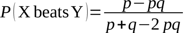
Equation 1
Here p is the winning percentage of team X and q is the winning percentage of team Y.1
Later in The Bill James Baseball Abstract of 1983, James extended the log5 method to individual player matchups. He credited Dallas Adams for the following equation, which evaluates the probability of a hit when batter X faces pitcher Y:
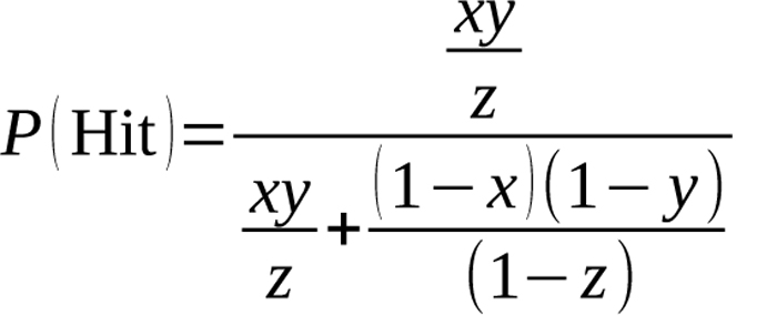
Equation 2
Here x is batter X’s batting average, y is the batting average of batters facing pitcher Y, and z is the batting average of the entire league.2
Both formulas have been observed to give accurate estimates of the probabilities for their respective events.3 As it is presented in James’ Abstracts, however, the log5 method can only estimate the probabilities for a sample space which contains two events—in the above examples, team X either wins or loses and a hit either occurs or does not. The log5 method does not necessarily hold as a probability function if a sample space is divided into more than two events such as the events of a single, double, triple, home run, etc. For this we must extend the method to apply to matchups consisting of two parties and a sample space partitioned into n parts.
By examining Equation (2) we can see how this extension of the log5 method might be accomplished. The numerator is made up of a three-variable term—the batter’s probability is multiplied by the pitcher’s probability and divided by the league average probability. For any event, we will refer to the value obtained from this relationship between the batter, pitcher, and league probabilities as the “base probability” of that event. The base probability alone is not sufficient, however, because the sum of all possible base probabilities may not equal one. Thus, we must normalize the base probability by dividing it by the sum of the base probabilities of all possible events. We can then imagine a general log5 formula that is similar to Equation (2), but with additional base probability terms in the denominator—one for each of the events into which the sample space is partitioned. In order to prove its mathematical basis, we will derive this general matchup probability formula and, by analyzing data from the 2012 MLB season, show that it is accurate when estimating the probabilities of a single, double, triple, home run, walk, hit-by-pitch, and out for a given batter-pitcher matchup.
Derivation of General Matchup Probability Formula
Let E1,…,En be events partitioning the sample space S of a given two-player matchup. Also let x={x1,…,xn} be the vector containing the event probabilities for Player 1 where xi is the probability of event i for i∈{1,2,…,n} , and let y={y1,…,yn} be the same for Player 2. Note that since the sample space is partitioned, x1+…+xn=y1+…+yn=1, and also P(E1)+…+P(En)=1.
We can imagine the matchup between Player 1 and Player 2 as a system where both players independently choose events based on their respective event probabilities. If both players select the same event, the system terminates. Otherwise it is restarted and both players choose again. This process continues until both players pick the same event.
Let the random variable I be the number of iterations the system goes through. Since we are now assuming the players choose events independently, the probability that both players select event i on the first iteration is given by
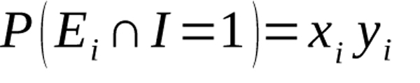
Equation 3
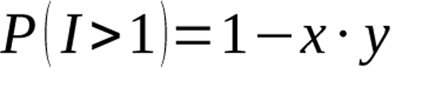
The probability that the system terminates after a single iteration is then given by
Equation 4
Thus, the probability the players choose different events and must choose again is
Equation 5
Iterations of the system are independent from one another, so we see that the probability that the system terminates with event i in k iterations is given by
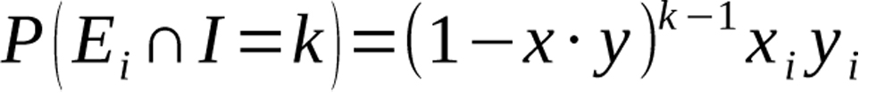
Equation 6
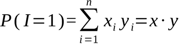
Summing over all possible values of k gives us the probability of event i:
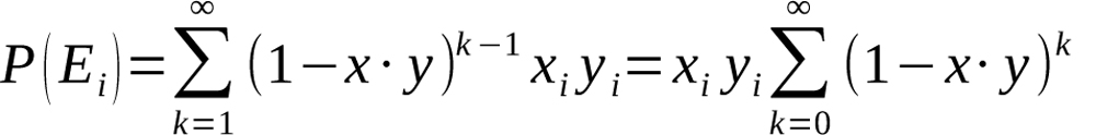
Equation 7
We now recognize that
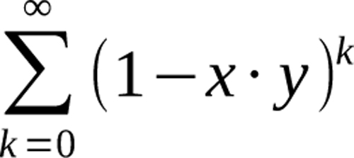
is a geometric series and will converge to
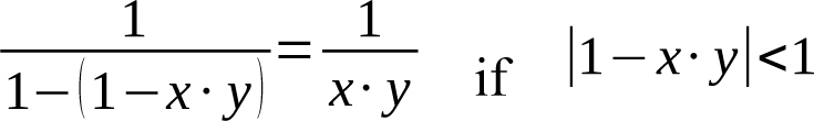
We know that 1−x⋅y is a probability, implying 0≤1−x⋅y ≤1. Therefore, the only way the convergence inequality would not be satisfied would be if 1−x⋅y=1 ⇔ x⋅y=0, in which case the system would never have terminated in the first place. Thus it is true that, barring a situation in which the system does not terminate, the series converges and we have
Equation 8
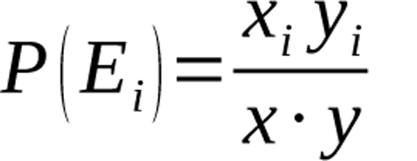
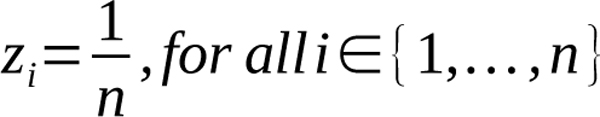
This assumes that the average player’s probability for each event is the same, i.e. all events have an equal probability of being selected if an event were to be selected at random. Of course this is not true of batter-pitcher matchups; an average batter facing an average pitcher is far more likely to hit a single than a triple, for example. To correct this, we must look at a player’s event probability relative to that event’s probability for an average player.
We introduce the vector z={z1,…,zn} which contains the event probabilities of an average player in the same way as x and y. It will later be shown that Equation (8) does not accurately predict matchup probabilities when the average probabilities for each event are not equal, and this modification is necessary to achieve an accurate prediction.
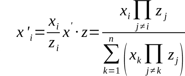
We now assume that Player 1’s event probabilities are in actuality the probabilities that each event occurs for Player 1 given that they are matched against an average player. We then wish to solve for the values x’i for i∈{1, 2,…,n} of x’={x’1,…,x’n}, a modified vector of Player 1’s event probabilities. For each of the n events, we get
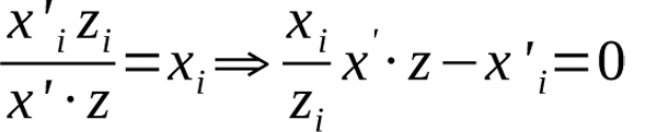
Equation 9
Notice that if we assume
and solve for x’i, we obtain the result x’i=xi:
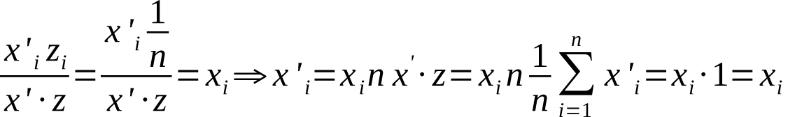
Equation 10
Now, adding the fact that x’1+…+x’n=1 to the conditions stated in Equation (9) and writing in vector notation, we obtain the following equation:
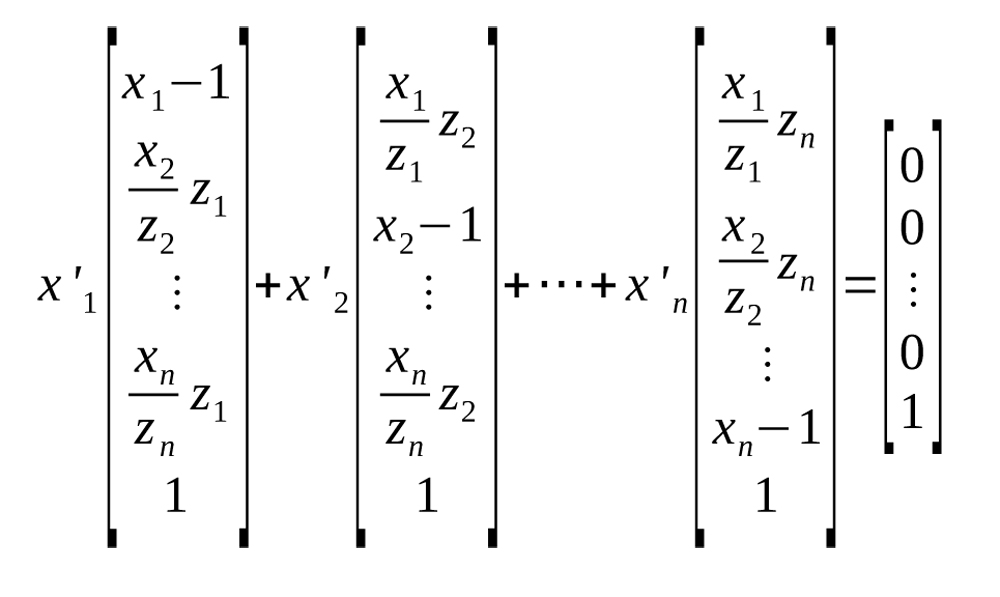
Equation 11
It can be shown that the solution for each x’i is
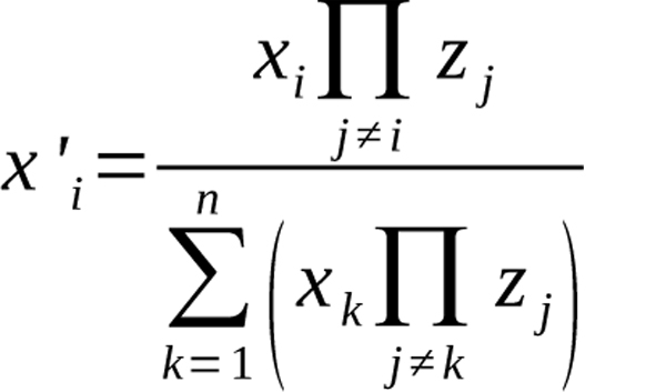
Equation 12
Now that we have a solution for x’1,…,x’n, we can replace x with x’ in Equation (8) and obtain
Equation 13
Justification of General Formula
In order to ensure that Equation (13) is, in fact, a probability function as we claim, we must make sure that
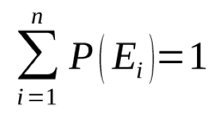
and also that 0≤ P(Ei )≤1, for all i∈{1,…,n}. Summing the probabilities of each event, we see that the total is one as expected.
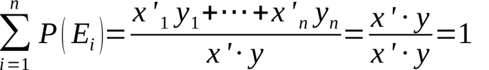
Equation 14
Furthermore, since every x’i and yi is a probability and therefore nonnegative, we can see by inspection that P(Ei)≥0. This fact also implies that P(Ei)≤1 since the denominator contains the numerator, plus other nonnegative terms.
Now that we have established that our formula is a probability function, there are a few more properties we must test to ensure it makes sense for estimating matchup probabilities. We expect, for example, that the probability event i occurs when Player 1 faces Player 2 would be the same as the probability of that event occurring when Player 2 faces Player 1. In other words, we want
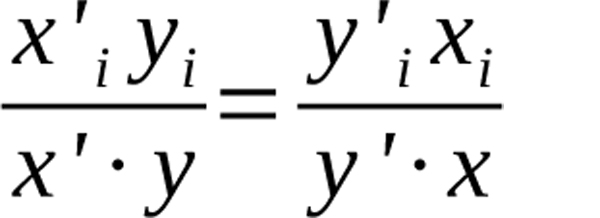
Equation 15
Indeed, this can be shown by substituting
into the above equation.
Notice that the relation in Equation (15) implies another property we would like our formula to satisfy—that an average player with probability vector z facing another player with probability vector x will return P(Ei)=xi. After modifying z to obtain z’ we get
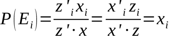
Equation 16
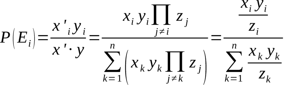
We will now show that the log5 method is a special case of our derived formula. Let the number of events n=2, and let z={z,1–z} be the vector containing the probabilities of events one and two for an average player, x={x,1–x} be the vector containing the event probabilities for Player 1, and y={y,1–y} be the vector containing the event probabilities for Player 2. Then by Equation (13) we have
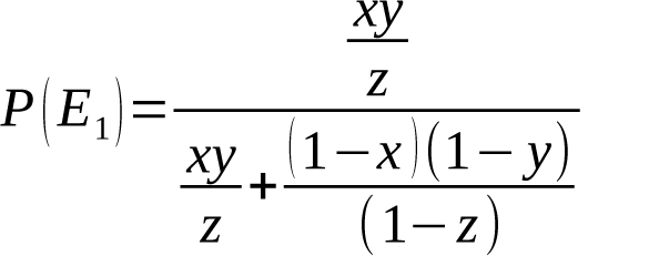
Equation 17
Notice that if we let x be the batting average of batter X, y be the batting average against pitcher Y, and z be the batting average of the entire league, this is the same formula seen earlier in Equation (2) for calculating the probability of a hit when batter X faces pitcher Y.
Furthermore, if we wish to interpret this expression as determining the probability that team X will beat team Y, we can let x be the probability team X wins, i.e. their winning percentage, and let y be the probability team Y loses, i.e. one minus team Y’s winning percentage. We then let z be the average winning percentage over the entire league. The value of z will necessarily be 0.5 since every time one team wins, another team must lose. Then, if team X has winning percentage p and team Y has winning percentage q we get
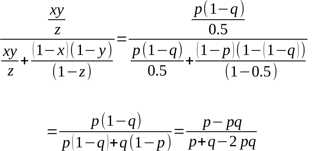
Equation 18
This, of course, is the log5 formula shown in Equation (1) to predict the probability that team X beats team Y given both team’s winning percentages.
Predicting Results of Batter-Pitcher Matchups
We will now use Equation (13) to predict the results of batter-pitcher matchups in Major League Baseball and compare our predictions to actual data obtained from the 2012 MLB season. In this situation, the sample space is plate appearances, each of which can result in a single, double, triple, home run, walk, hit-by-pitch, error, sacrifice hit, sacrifice fly, fielder’s choice, catcher’s interference, or out. The batter will be called out if an out, sacrifice hit, or sacrifice fly occurs. Additionally, an error is recorded only if the batter would have been called out had an error not occurred. Likewise, fielder’s choice denotes that the batter could have been thrown out, but the fielder instead elected to throw another runner out. For the sake of simplicity, we can combine the events of an out, sacrifice hit, sacrifice fly, error, and fielder’s choice under the event out, which we will interpret as the event that the batter is called out or would have been called out under normal circumstances.
We will now take into account another factor. The circumstances governing when pitchers intentionally walk batters are not solely based upon the ability of the pitcher or batter, but upon factors that are outside the realm of the batter-pitcher matchup, such as the configuration of baserunners, the number of outs, etc. In the same way, catcher’s interference is the result of outside influences acting upon the matchup. For this reason, we will ignore intentional walks and catcher’s interference. For the remainder of this article, unless otherwise specified, the terms “plate appearances” and “batters faced” will refer only to those that did not result in an intentional walk or catcher’s interference, and “walks” will refer only to unintentional walks.
We therefore have that each plate appearance can be one of seven distinct events: a single, double, triple, home run, walk, hit-by-pitch, or out. Let these correspond to events one through seven respectively. Probabilities of these events occurring for a given batter can then easily be calculated by dividing the number of times the event occurred during one of his plate appearances by his total number of plate appearances. The same can be said for a pitcher if we divide the number of times each event occurred after one of his pitches by the total number of batters he has faced.
We use event files obtained from Retrosheet to count the number of singles, doubles, triples, home runs, walks, hit-by-pitches, outs,4 and plate appearances/batters faced for individual players during the 2012 MLB season. These event files contain a play-by-play account of all games during an entire season including the information we are interested in—the pitcher, batter, and result—as well as other information such as the score, number of outs, and baserunner configuration.
We then look only at batters who have at least 502 plate appearances and pitchers who have faced at least 502 batters, this time including intentional walks. This number was chosen because 502 is the minimum number of plate appearances to be eligible for the Major League Baseball batting title. This restriction leaves us with 144 batters and 124 pitchers.5 During the 2012 season, these 144 batters faced these 124 pitchers a total of 44,209 times.6
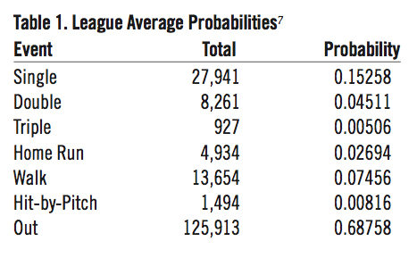
We then must find the sample proportion and number of occurrences we expect for each event if our formula for determining batter-pitcher matchup probabilities in Equation (13) is true. In the 2012 season there were a total of 183,124 batters faced, the distribution and league average probabilities of which are shown below in Table 1.
We now have all the variables necessary to use Equation (13) to find the probability of event i for each batter-pitcher matchup. Let B be the set containing the batters with at least 502 plate appearances and P be the set containing all the pitchers with at least 502 batters faced. Then B x P is the set containing all possible matchups between the batters in B and pitchers in P. Let Nl,k be the total number of times batter l faces pitcher k. The expected number of occurrences of event i is then
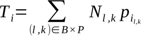
Equation 19
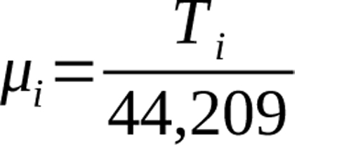
where Pilk is the probability of event i when batter l faces pitcher k. The expected sample proportion of event i is then
Equation 20
Now that we have the expected sample proportion and number of occurrences for each event, we can perform a one-proportion Z-test with significance level α=0.1 to determine the probabilities that the sample proportions and expected sample proportions are equal. The results are summarized in Table 2.
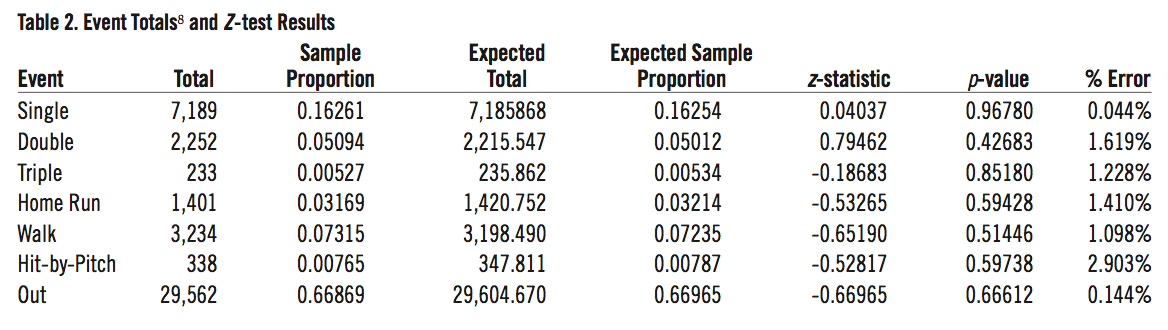
We also perform a χ2 test with six degrees of freedom and significance level α=0.1 to determine whether the distribution of the seven events is consistent with our expected distribution. This test yields a χ2 statistic of approximately 1.64, and the probability of observing this or a more extreme difference in expected and observed totals is 0.95.
Note that if we were to use Equation (8) to calculate the event probabilities for each batter-pitcher matchup, we would obtain the results in Table 3.
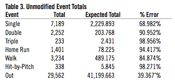
A χ2 test with significance level α=0.1 of the above data yields a χ2 statistic of 113,417.71. Consultation of the χ2 distribution for six degrees of freedom shows the probability of observing this difference is zero, and we can safely accept the alternative hypothesis that Equation (8) does not accurately predict these matchup probabilities.
Specific Batter-Pitcher Matchups
Perhaps the most intriguing aspect of our formula is its ability to predict the results of specific batter-pitcher matchups. Alex Gordon faced Chris Sale a total of 22 times during the 2012 season, the most that any one batter faced any one pitcher in the 44,209 plate appearances selected for our sample. Using Equation (13) we can compare the expected results of Alex Gordon’s 22 plate appearances against Chris Sale to what actually occurred.
The relevant statistics from the 2012 season for Alex Gordon and Chris Sale are shown below in Table 4:
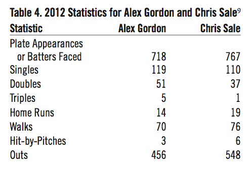
Using the above numbers to seed Equation (13) gives us the probabilities for each of the seven events. Finally, we multiply each of these probabilities by 22 to obtain the expected number of occurrences for each event in 22 matchups between Gordon and Sale.
Rounding our expected results, we see that in 22 plate appearances against Chris Sale, we would expect Alex Gordon to hit about three singles, two doubles, zero triples, zero home runs, be walked twice, hit by a pitch zero times, and called out 15 times. This is almost exactly what occurred. Gordon instead hit four singles, two doubles, zero triples, zero home runs, was walked once, hit by a pitch zero times, and called out 15 times—the only difference being that Gordon hit one more single and was walked once less than expected.
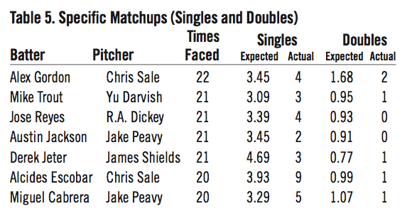
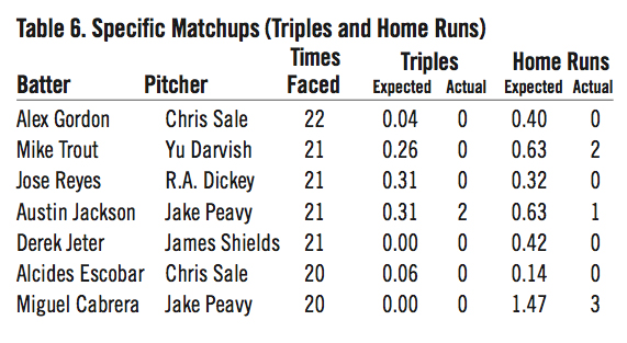
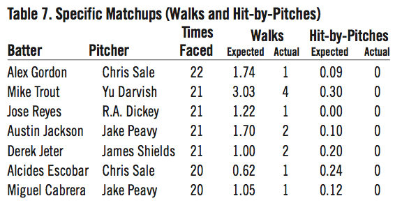
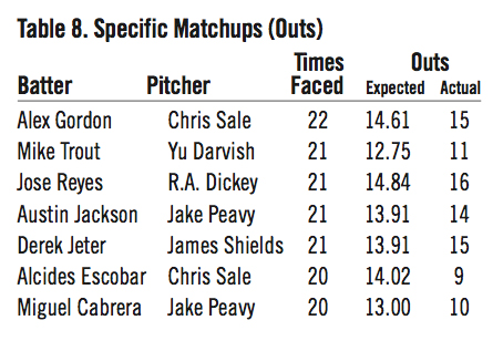
In fact, seven batter-pitcher matchups in our 44,209-plate appearance sample occurred at least 20 times. The expected and actual results of these matchups are summarized in Table 5 through Table 8 below.7 Note that with such a small sample size for each matchup, the results cannot be considered conclusive and are presented for illustrative purposes only.
Conclusion
The general matchup formula shown in Equation (13) seems to be a good estimator of batter-pitcher matchup probabilities. All p-values shown in Table 2 are greater than 0.1, so we reject the hypothesis that the proportions for each event are unequal. That is, the data do not support the claim that the proportions are unequal. Likewise, the result of the χ2 test indicates we cannot conclude that the distributions are unequal and must accept the null hypothesis that the distributions are the same. These tests, along with the small margin of error for each of the seven events, suggest that the formula in Equation (13) can be used to accurately predict the probabilities of the results of a batter-pitcher matchup.
MATT HAECHREL received his Bachelor of Science in Mathematics from the University of Minnesota in 2013. He currently resides in the Minneapolis-St. Paul area where he works as a contract analyst. This article is a revised edition of his senior thesis which was submitted to the University of Minnesota Honors Program in May 2013. Matt would like to thank Lawrence Gray and Matthew Danielson for their valuable guidance throughout the process of completing this paper. He may be contacted at haechrelmatt@gmail.com.
Sources
James, Bill. “Pythagoras and the Logarithms.” Baseball Abstract, 1981: 104–110.
James, Bill. “Log5 Method.” The Bill James Baseball Abstract, 1983: 12–13.
Levitt, Dan. Baseball Think Factory, “The Batter/Pitcher Match Up.” Last modified November 4, 1999. Accessed April 27, 2013. http://www.baseballthinkfactory.org/btf/scholars/levitt/articles/batter_pitcher_matchup.htm.
Miller, Steven J. Brown University, “A Justification of the log5 Rule for Winning Percentages.” Last modified April 20, 2008. Accessed April 27, 2013. http://web.williams.edu/Mathematics/sjmiller/public_html/103/Log5WonLoss_Paper.pdf.
Retrosheet, “Play-by-Play Data Files (Event Files).” Last modified December 6, 2012. Accessed January 16, 2013. http://www.retrosheet.org/game.htm
Sports Reference LLC, “Baseball-Reference.com.” Accessed May 6, 2013. http://www.baseball-reference.com.
Tippett, Tom. Diamond Mind, Inc., “May the best team win…at least some of the time.” Last modified October 1, 2002. Accessed April 27, 2013. http://207.56.97.150/articles/playoff2002.htm.
Notes
1 Bill James, “Pythagoras and the Logarithms,” Baseball Abstract, 1981: 104–10.
2 Bill James, “Log5 Method,” The Bill James Baseball Abstract, 1983: 12–13.
3 Dan Levitt, “The Batter/Pitcher Match Up,” Baseball Think Factory, last updated November 4, 1999, http://www.baseballthinkfactory.org/bt/scholars/levitt/articles/batter_pitcher_matchup.htm; Tom Tippett, “May the best team win…at least some of the tme,” Diamond Mind, Inc., last updated October 1, 2002, http://207.56.97.150/articles/playoff2002.htm.
4 Outs here include the Retrosheet events of generic outs, strikeouts, errors, and fielder’s choice. Sacrifice hits and sacrifice flies are subsets of generic outs.
5 “Baseball-Reference.com,” Sports Reference LLC, accessed May 6, 2013, http://www.baseball-reference.com.
6 “Play-by-Play Data Files (Event Files),” Retrosheet, accessed January 16, 2013, http://www.retrosheet.org/game.htm. This does not include instances when the result of the plate appearance was an intentional walk or catcher’s interference.
7 “Play-by-Play Data Files (Event Files),” Retrosheet, accessed January 16, 2013, http://www.retrosheet.org/game.htm. Actual results data from Tables 5, 6, 7, and 8 come from this source.