
The PING Ratings: A Model for Rating NCAA Baseball Teams
This article was written by Philip Yates
This article was published in Fall 2011 Baseball Research Journal
BACKGROUND
In 2008 the Fresno State Bulldogs beat the heavily favored Georgia Bulldogs in the NCAA College Baseball World Series. That Fresno State squad finished with a 47–31 record, the most losses ever for an NCAA baseball champion. The Bulldogs were the fourth seed in their regional with Long Beach State as the top seed. They met Arizona State, the number three national seed, in the super regionals. Only four teams play in each of 16 regionals. This would be the equivalent of a team seeded 13th winning the NCAA men’s basketball tournament. It is safe to say that they were the lowest seed in any sport to win an NCAA championship.
Over the past few seasons, college baseball has begun to gain in popularity. ESPN has started to air the NCAA College Baseball Regionals selection show. Various internet message boards debate the selection of some teams over others just like with the NCAA Division I college basketball tournament. With this increase in popularity and scrutiny over the selection of teams, improvements in the ranking of NCAA baseball teams may be needed.
When constructing a ranking system of individuals or teams, some issues need to be addressed. Danehy and Lock (1995) say that any ranking system should order all teams, compare teams, adjust for the quality of the opponents, predict outcomes of games, and predict the game scores and differentials.[fn]Timothy J. Danehy and Robin H. Lock, “CHODR—Using Statistics to Predict College Hockey,” STATS: The Magazine for Students of Statistics (1995), Vol. 13, 10–14.[/fn] Statistical methods to rank teams have been widely used in sports. The following is just a brief list of some of the work that has been done in the past. Harville applied linear-model methodology to the point spread of games in college football.[fn]David Harville, “The Use of Linear-Model Methodology to Rate High School or College Football Teams,” Journal of the American Statistical Association (1977), Vol. 72, 278–289.[/fn] This methodology can be applied to high school football. Stern (1995) used a least-squares approach to rank college football teams. Danehy and Lock (1995) used an additive least squares model and Lock and Danehy (1997) used a multiplicative Poisson model for collegiate hockey rankings.[fn]Robin H. Lock and Timothy J. Danehy, “Using a Poisson Model to Rate Teams and Predict Scores in Ice Hockey,” American Statistical Proceedings of the Section on Statistics in Sports (1997), 25–30.[/fn] Glickman and Stern developed a predictive model based on a state-space model that assumes team strengths follow a first-order autoregressive process.[fn]Mark E. Glickman and Hal S. Stern, “A State-Space Model for National Football League Score,” Journal of the American Statistical Association (1998), Vol. 93, 25–35.[/fn] Annis and Craig used a hybrid paired comparison model that incorporates wins and scores to rank college football teams.[fn]David H. Annis and Bruce A. Craig, “Hybrid Paired Comparison Analysis, with Applications to the Ranking of College Football Teams,” Journal of Quantitative Analysis in Sports (2005), Vol. 1, No. 1, Article 3.[/fn] Kvam and Sokol presented a combined logistic regression/Markov chain model that was applied to NCAA basketball data in order to predict the NCAA basketball tournament games.[fn]Paul Kvam and Joel S. Sokol, “A Logistic Regression/Markov Chain Model for NCAA Basketball,” Naval Research Logistics (2006), Vol. 53, 788–803.[/fn]
Govan, Langville, and Meyer use an Offense-Defense model to rank teams in college basketball, college football, and the NFL.[fn]Anjela Y. Govan, Amy N. Langville, and Carl D. Meyer, “Offense-Defence Approach to Ranking Team Sports,” Journal of Quantitative Analysis in Sports (2009), Vol. 5, No.1, Article 4.[/fn]
Previous work in ranking college baseball teams exists on a few web pages. Boyd Nation publishes his ISR (Iterative Strength Ratings) on his website.[fn]Boyd Nation, “Boyd’s World,” http://boydsworld.com (1998).[/fn] Nation uses an algorithm to combine a team’s winning percentage with their strength of schedule. The goal of the ISR is to take advantage of inter-regional games more accurately than other systems. Warren Nolan has a ranking system called NPI.[fn]Warren Nolan, “College Sports,” http://warrennolan.com (2004).[/fn] Nolan keeps his ranking system secret. There is no glimpse on how the NPI is calculated. Both Nation and Nolan compare their rankings to the RPI. The RPI (Ratings Percentage Index) is the ranking system that the NCAA uses for teams in college basketball and baseball. Although there are websites that publish an RPI, all of these are approximations of what the NCAA actually does. The NCAA keeps their adjustments to the RPI secret.
This paper will focus on a ranking system that will be referred to as the PING (Power Index Ratings) ratings. Specifically, a least-squares approach similar to Stern (1995) will be used. Instead of the difference in runs between the two teams, the difference in Base Runs will be the response for the PING ratings model. The model will be applied to data from the 2009 NCAA baseball season. Only games between Division I teams will be considered.
DATA AND THE MODEL
The Data
The response for the PING ratings model is a difference in Base Runs between the home and away teams. Base Runs first appeared in David Smyth’s Base Runs Primer in the early 1990s. Unfortunately, the primer is no longer available online. It was designed to estimate the number of runs a team should have scored in a game given their offensive statistics. Base Runs help to remove the luck factor involved by attempting to disregard the order in which the team’s hits and walks came within an inning. Currently, Tango has the best introduction to the concept of Base Runs.[fn]Tom Tango, “Base Runs—Sabermetrics,” www.tangotiger.net/wiki/index.php?title=Base_Runs (2008).[/fn]
The reason Base Runs excel at predicting under normal circumstances as well as extreme cases is that they make reasonable assumptions about how runs are scored. The first assumption is that each batter will make an out, hit a home run, or reach base safely. When a batter reaches base safely, he will then either score, make an out on the bases, or be left on base when the inning is over. There will be four factors that will be used in the calculation of Base Runs. Heipp describes the factors in the following manner. Factor A represents final baserunners. These players reach base either by hit or walk. Home runs are subtracted out since the batter never reaches base. Factor B represents the advancement of those runners. It includes all events except for outs. The coefficients in factor B are intrinsic linear weights. Factor C represents outs made by batters. Factor D consists of only home runs.[fn]Brandon Heipp, “Buckeyes and Sabermetrics: Base Runs,” http://gosu02.tripod.com/id108.html (2004).[/fn]

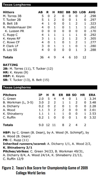
According to Tango (2008), Smyth came up with three basic equations to compute Base Runs. The most basic version is
where H are hits, BB are walks, HR are home runs, TB are total bases, and AB are at bats.
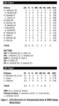
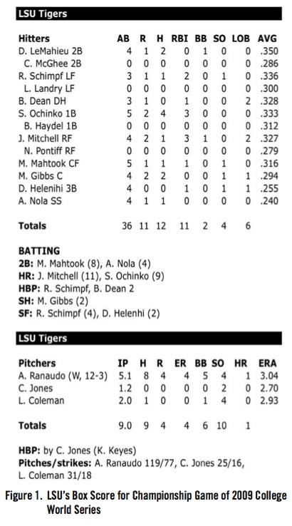
Figures 1 and 2 show the box score for the last game of the 2009 NCAA College World Series played at Rosenblatt Stadium in Omaha, Nebraska on June 24, 2009 between the Louisiana State University Tigers and the University of Texas Longhorns. The Base Runs would be calculated in the following manner. For LSU,
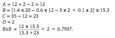
For Texas,
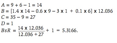
Since this game was played on a neutral field, the prediction is that LSU would win the game by 1.3552 Base Runs. The actual score was LSU 11, Texas 4. Clearly, LSU was more efficient at scoring runs, i.e. scoring more runs than what was expected of them, than Texas in the final game.
THE MODEL
The model used to produce the PING ratings is a variation of the method developed by Stern (1995) to rate college football teams as well as predict individual game outcomes. The goal of the ratings is to account for the team’s performance and their strength of schedule.
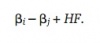
A method of least squares approach is used to create the ratings. Let ßi be the unknown rating for team i, ßj be the unknown rating for team j, and HF denote the home field advantage. The outcome Yk represents the difference in Base Runs between the home team and road team in the game number k. The expected outcome if team i plays team j on team i’s home field would be
The actual outcome will usually differ from this expected outcome. For college football, Stern (1995) proposed to minimize the sum of squares between these two values. For college baseball, this similar technique will be used to determine the values of ßi, ßj, and HF, which minimize
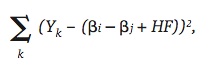
where i = 1,…,302, j = 1,…,302, i ? j, k is the game number, which goes from 1 to 8,258 for the 2009 season, and HF is set to 1 if there is a home team and 0 if the game is played on a neutral field. The ß’s can be coded as 1 or –1 depending if the team is the home team (1) or the road team (–1). If the game is at a neutral site, there must be one ß to be coded as 1 and the other as –1.
One problem that Stern (1995) had to deal with when constructing his rating system for college football was the presence of outliers. Traditionally in collegiate athletics, when a team from an upper division plays a team from a lower division, the outcome is lopsided. This phenomenon can occur even when the two teams are from the same division, i.e. Division I, but from different conferences. For example, a team from the SEC (Southeastern Conference), considered a top conference for NCAA baseball, would be expected to beat a team from the America East conference, considered a weaker conference for NCAA baseball, by a large margin. Stern used an adjusted outcome when the margin of victory was beyond 20 points.[fn]Hal S. Stern, “Who’s Number 1 in College Football? …And How Might We Decide?” CHANCE (1995), Vol. 8, No. 3, 7–14.[/fn] The modified outcome was equal to 20 points plus the square root of the additional margin of victory beyond 20 points. The question still remains: what is considered a lopsided victory in NCAA baseball? Since the outcome for the PING ratings is the difference in Base Runs for the home and road teams, the answer to the question is not a simple one.
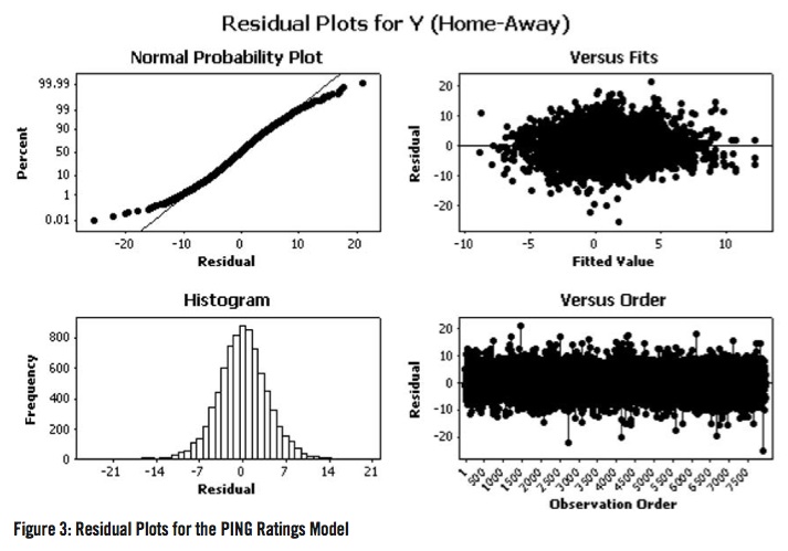
The model for the PING ratings was run for all 302 NCAA Division I baseball teams. Figure 3 shows the residual plots for the PING ratings model with no adjustment for blowouts. Even though there is no parametric assumption being made with the PING ratings model, the normal probability plot can be used as an “ad-hoc” tool for deciding what a lopsided victory is in terms of Base Runs for NCAA baseball. The “departure” from normality seemed to occur around 9 Base Runs.
In order to adjust for the impact of blowouts on the PING ratings, games with differences of Base Runs of at least 9 will be controlled for in the following manner. Nine Base Runs will be subtracted from the actual difference in Base Runs. This new difference will be halved and added to the nine Base Runs:
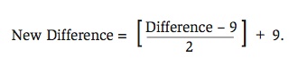
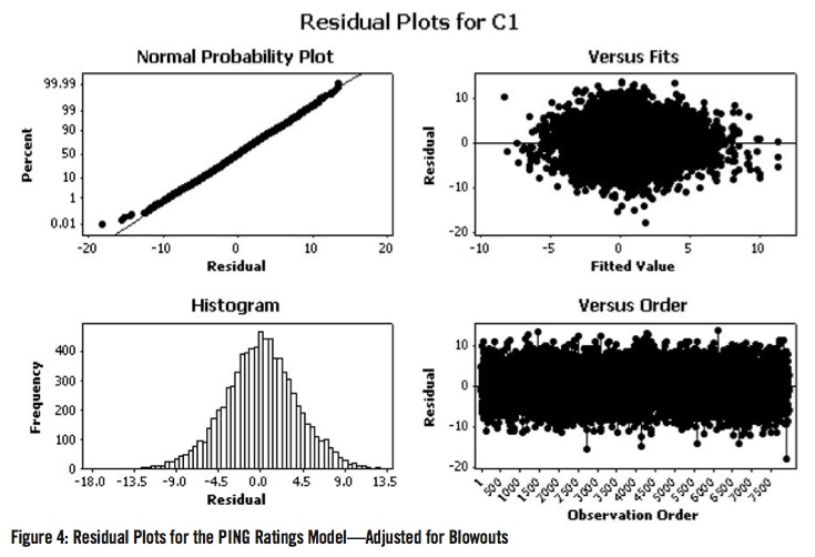
For example, a victory by 21 Base Runs will be reduced to a victory by 15 Base Runs. Figure 4 shows the residual plots for the PING ratings model after the adjustments for blowouts were made. While there is no theoretical justification for this exact adjustment other than to adjust Base Runs in a manner different from the modification proposed by Stern (1995), Figure 4 indicates that this adjustment in the difference of Base Runs is yielding outcomes that one would expect if normality were assumed.
RESULTS
Going into the 2009 NCAA Division I Baseball Championships on May 29, 2009, the PING ratings were used to predict the winners of the regional, super regional, and College World Series games. The championships behave a bit differently than the NCAA Division I Basketball Tournament. There are 16 regionals each featuring four teams. The teams play in a double elimination format. The last team remaining advances to the super regionals. The super regionals are a best of three format. The last eight teams remaining advance to the College World Series in Omaha, Nebraska. The College World Series is a double elimination format. The last two teams remaining then play each other in a best of three format for the national championship.
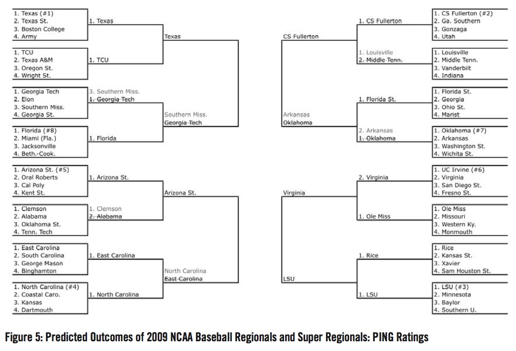
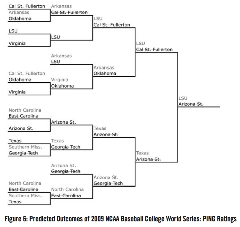
Figure 5 shows the predicted outcomes of the 2009 NCAA Division I Baseball regional and super regional games. The PING ratings correctly picked 12 of the final 16 teams and 5 of the 8 College World Series teams. Southern Mississippi’s making the 2009 College World Series was a shock to the majority of pundits since they were the third-ranked team in their region. This is analogous to an eleven seed making it to the Elite Eight in the NCAA Basketball Tournament. Overall, the PING ratings picked Arizona State to beat Cal State Fullerton in the College World Series championship game. These results can be found in Figure 6. Due to the double elimination nature of the College World Series, the PING ratings’ results look worse than they are. In the “Final Four” of the College World Series, two Texas Longhorns players (catcher Cameron Rupp and center fielder Connor Rowe) hit solo home runs in the bottom of the ninth to beat Arizona State 4–3. That was the elimination game for the PING rating’s champion.
(Click image to enlarge)
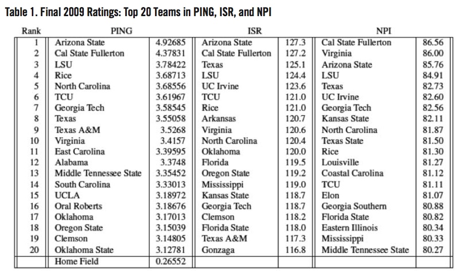
Table 1 lists the final ratings for the top 20 teams in the PING ratings, Boyd Nation (1998)’s ISR ratings, and Warren Nolan (2004)’s NPI rankings. One possible way to compare the three rating systems is to find the correlation for each one with RPI. Although it is not a flawless ranking system, the RPI is one of the criteria the NCAA uses to select teams for the NCAA College World Series. All of the rating systems had roughly the same correlation with RPI: PING (r=0.81), ISR (r=0.83), and NPI (r=0.84).
The PING ratings had the 2009 National Champion LSU Tigers rated the highest out of the three ratings systems, though to be fair, the difference is small (#3 versus #4); however, for a given game, the ratings would predict that LSU would lose at home to Cal State Fullerton by 0.32857 Base Runs (4.37831– (3.78422+0.26552)) and to Arizona State by 0.87711 Base Runs. The eight teams to actually participate in the 2009 NCAA College World Series were LSU, Texas, Arkansas, Arizona State, Virginia, North Carolina, Cal State Fullerton, and Southern Mississippi. The final PING ratings had five of those eight teams in the top eight. The ISR and NPI ratings had similar results.
Where did these rankings go wrong? For the PING ratings, UCLA is a surprising entry at number 15. The 2009 UCLA Bruins finished with a 27–29 record against Division I teams and failed to make the NCAA baseball tournament. According to Nolan (2004), UCLA had the 28th most difficult schedule in all of college baseball. For the NPI ratings, Eastern Illinois (#18) failed to make the NCAA baseball tournament. The EIU Panthers finished 36–14 against Division I teams; however, they failed to make the NCAA baseball tournament. Nolan (2004) had EIU with the 192nd most difficult schedule in college baseball. Losing in the Ohio Valley Conference tournament was the reason why they did not make the cut. Eastern Illinois finished 49th in the PING ratings.
SUMMARY and CONCLUSIONS
The combination of Base Runs and least squares methods can be used to properly rate college baseball teams. However, there is plenty of room for improvement for the PING ratings. The calculation of Base Runs presented by Tango (2008) is best used for Major League Baseball. With proper play-by-play data from college baseball, perhaps the coefficients used to calculate A, B, C, and D can more accurately reflect what is going on in NCAA Baseball. Unfortunately, this play-by-play data is not easy to track down like it is for Major League Baseball. Other possible future work could be the incorporation of a measure for the streakiness of a team, i.e. how is the team playing over their last 10 games. LSU came into the tournament playing very well. They finished their season by winning 15 of their last 17 games. Being able to account for the streaks may have meant the difference of LSU finishing third and finishing first in the PING ratings. Some may argue that a flaw in the PING ratings is the failure to account for pitching; however, it should be noticed that the other methods (ISR and RPI) only look at winning percentages and strength of schedule. Again, it is kind of a secret as to how NPI is calculated. None of those three methods (ISR, NPI, RPI) are used to predict outcomes.
PHILIP YATES is an assistant professor of mathematics at Saint Michael’s College in Colchester, Vermont. His analysis of hitting streaks with David Rockoff appeared in “Journal of Quantitative Analysis in Sports” and “CHANCE”. Philip has been a member of SABR since 2007. He would also like to add, “Go, Cubs, go!” Since he graduated from the University of South Carolina, for this paper it is more appropriate to say “Go Gamecocks!”
ACKNOWLEDGEMENTS
I would like to thank my student, Edward Reyes, for all of his help with the data entry for the 2009 NCAA season. Thanks to David Rockoff for his comments and feedback with the initial draft of this paper.