

Probabilities of Victory in Head-to-Head Team Matchups
This article was written by John A. Richards
This article was published in Fall 2014 Baseball Research Journal
Winning percentages represent the fundamental metric of team success. Regardless of a team’s specific strengths and weaknesses, its winning percentage—or equivalently, its won-lost record in a fixed-length season—is the ultimate distillation of all other individual and team statistics into a single measure of success or failure. Winning percentages determine which teams advance to the postseason and largely define teams’ legacies. And among teams playing a balanced schedule in the same league, winning percentage provides an unambiguous gauge of relative team strength: won-lost record is taken as the ultimate arbiter of team quality and the final yardstick by which to differentiate teams. Even if we grant that luck plays a role in every season, and that the vagaries of chance may render absolute team quality ultimately unknowable, we accept that a team’s final won-lost record provides the best observable record of this quality relative to the league in which that team played.
Winning percentage not only measures team success, but also serves an important predictive function. When two teams meet for a game, we generally expect the team with the higher winning percentage to have a greater probability of victory. Furthermore, we expect each team’s probability of victory in a head-to-head matchup to depend on the similarity or dissimilarity of their winning percentages. We might ask, however: can this general qualitative expectation be formalized quantitatively? Can it be refined to the point of mathematical specificity, such that the probability of each team’s victory in any head-to-head matchup might be expressed as a function of the contesting teams’ winning percentages?
This article examines the relationship between teams’ winning percentages and their probabilities of victory in head-to-head matchups. We present a thought experiment that suggests a mathematical expression for the probability of each team’s victory given their winning percentages, and we compare this expression and its derivation to a previously proposed formula. We calculate historical head-to-head winning percentages for all games throughout major league history and show that the predictions of our proposed equation are in agreement with these empirical results. Finally, we suggest a minor refinement to the proposed formula that yields enhanced predictive power and even better agreement with empirical results. Please note that for purposes of this paper, we use the term “winning percentage” in the vernacular sense, presenting the “percentages” as averages akin to batting average, a decimal followed by three places. A team with a “winning percentage” of .600 has won 60 percent, not six-tenths of a percent, of its games.
A Thought Experiment
Suppose that two teams—Team A and Team B—play the same balanced schedule in the same league. During spring training, Team A and Team B agree to meet after the conclusion of the season to stage a single post-season exhibition game. Unfortunately, they fail to consider which team will host the contest. As the season progresses, the question of venue becomes a sticking point. By the end of the season, the issue has become so contentious that the A’s and the B’s both refuse to meet on any field for the proposed post-season game, and it appears the contest will have to be called off.
Enter Team C, which has finished the season with a .500 record. Team C proposes a novel solution that will enable either Team A or Team B to legitimately claim victory in a hypothetical A-vs.-B matchup without ever setting foot on the same diamond at the same time. They propose that all three teams—A, B, and C—travel to a neutral site and play a series of games that will serve as a proxy for the now-untenable single-game matchup between Team A and Team B. In particular, Team C proposes playing a single game against Team A and a single game against Team B. They propose that the outcome of this two-game “proxy series” be used to assign victory according to the following common-sense rules:1
1. If A defeats C and C defeats B, then A is declared the victor over B.
2. If B defeats C and C defeats A, then B is declared the victor over A.
3. If A and B both defeat C, or if C defeats both A and B, then no victor is yet declared.
Team C further proposes that in case of outcome 3, the two-game series will be repeated—recursively, if necessary—until outcome 1 or 2 is achieved, and Team A or Team B is declared the victor accordingly. Note that outcomes 1 and 2 in Team C’s proposal are decisive in the sense that they allow a definitive ordered ranking of the three teams—and thus of Team A and Team B. In contrast, outcome 3 is not decisive because it does not allow a definitive ordered ranking of Teams A and B relative to each other. Outcome 3 thus necessitates one or more additional two-game series(repeated until either outcome 1 or 2 is realized) to achieve a decisive ordered ranking.
Because Team C is exactly a league-average team—that is, they possess exactly a .500 record after playing a balanced schedule within the league—all three teams agree that this proxy series is a fair and unambiguous way of declaring a victor in lieu of an actual head-to-head matchup between Team A and Team B. The A’s, B’s, and C’s travel to a neutral site to play their two-game proxy series (as well as any subsequent two-game proxy series necessitated by outcome 3) that will ultimately crown Team A or Team B the victor without requiring a head-to-head contest.
Derivation of a Win Probability Function
The proxy series described in this thought experiment provides an unbiased method for assigning victory to one of two teams without requiring a head-to-head matchup. As it turns out, the proxy-series formulation also lends itself directly to the derivation of a functional expression for each team’s probability of victory in such an event, given their full-season winning percentages. Let us denote the winning percentages of Team A and Team B by WPA and WPB, respectively. Note that WPA and WPB represent winning percentages achieved in the context of a full league playing a balanced schedule. Because the proxy Team C achieved a winning percentage of exactly .500 playing the same balanced schedule in the same league, it stands to reason that Team A and Team B should expect to win individual games against Team C with probabilities WPA and WPB, respectively. If individual games of the proxy series are assumed independent, then the probabilities of each of the three possible outcomes of the two-game series can be expressed directly. In particular, the probability of Team A achieving victory (outcome 1) in a single two-game proxy series is

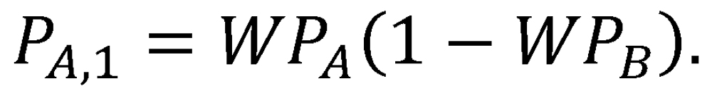
(The “1” in the subscript indicates that this outcome was achieved after a single two-game proxy series with no rematch; this notation will be useful in the derivation that follows.) Similarly, we can write the probability of Team B achieving victory (outcome 2) after a single two-game proxy series as

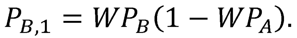
Finally, the probability of no decisive victory (outcome 3) after a single two-game proxy series is


The probabilities of the three possible outcomes can be depicted graphically on the unit square, as in Figure 1. This square is divided into four regions by one vertical line (corresponding to the winning percentage of Team A) and one horizontal line (corresponding to the winning percentage of Team B). The areas of the resulting regions are equal to specific probabilities expressed in the above set of equations. In particular, the two white regions have areas equal to the probabilities of the decisive outcomes 1 and 2 (that is, PA,1 and PB,1), while the union of the two shaded regions has an area equal to the probability of the nondecisive outcome 3 (that is, P0,1).

Figure 1 (click to enlarge)
Because a single two-game proxy series may not be decisive (outcome 3), a recursive sequence of two-game proxy series might be required to declare a victor. The probability of Team A achieving victory in a sequence of n or fewer proxy series is


Likewise, the probability of a victory for Team B after n or fewer two-game proxy-series recursions is


Finally, the probability of no decisive outcome after a sequence of n recursive two-game proxy series is

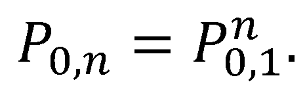
(It can be verified that PA,n + PB,n + P0,n = 1 for any n.)
As n increases, the probability P0,n of having reached no decisive outcome decreases toward zero and the probabilities PA,n and PB,n of having reached each decisive outcome increase toward a sum of one. In the limiting case—that is, as n tends to infinity—a decisive result will be achieved with probability one. Summing the resulting arithmetic series, we find that the probability of eventual victory for team A is2

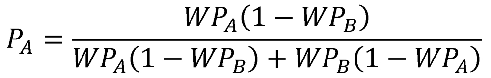
and the probability of eventual victory for Team B is

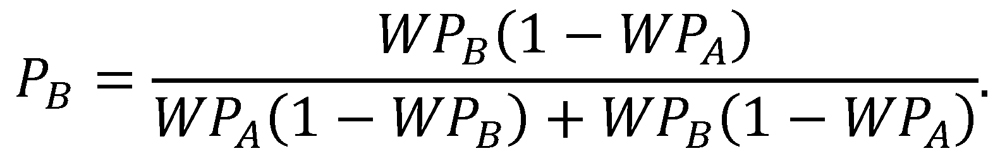
Note that PA is simply the ratio of PA,1 to the sum PA,1 + PB,1, and that PB is likewise the ratio of PB,1 to the same sum. In other words, the probability of each team’s victory is simply the ratio of its probability of victory in a single two-game proxy series to the probability of a decisive result in a single two-game proxy series. Because the equations for PA and PB are complementary, we will henceforth represent them with a single function of the two variables WPA and WPB:
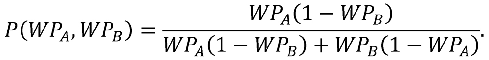

Here, P(WPA,WPB) represents the probability of a victory by Team A over Team B, given that these teams have inherent qualities of WPA and WPB, respectively.3 Note that PA = P(WPA,WPB) and PB = P(WPB,WPA).
We contend that the function P describes not only the probability of team victory in a proxy series, but also in an actual head-to-head matchup. That is, we maintain that if Team A and Team B met directly, without the artifice of a proxy series with Team C, then P would express the win probability for each team. It is easy to verify that P satisfies a number of intuitive criteria that we would demand of any function claiming to predict the probability of victory in head-to-head matchups. In particular:
• P(x,y) = 1 – P(y,x); equivalently, P(x,y) + P(y,x) = 1. A matchup between two teams must result in a victory for one of the teams.
• P(x,.500) = x. A team with winning percentage x will also have winning percentage x against a league-average team.
• P(x,x) = .500. A matchup between two teams with the same winning percentage is equally likely to result in victory for either team.
• P(x,0) = 1 for all x > 0. A team with a nonzero winning percentage is certain to defeat a team that has no probability of winning.
• P(x,1) = 0 for all x < 1. A team with a subunity winning percentage is certain to lose to a team that has no probability of losing.
• P(x+d,y) > P(x,y) for all d > 0 and 0 < y < 1. As a team’s winning percentage increases, its probability of victory against any opponent also increases (unless that opponent has winning percentage 0 or 1).
Indeed, these precepts are so basic and self-evident that they might actually be used (possibly with other criteria) to construct the function P on an axiomatic basis.
Table 1 presents the predicted probabilities of victory in head-to-head matchups between teams of different qualities. Each cell in the table represents the predicted probability of victory for a team with quality indicated by the heading of the corresponding row, when facing a team with quality indicated by the heading of the corresponding column.4 For instance, the predicted probability of victory for a .600 team facing a .400 opponent is .692. When the same .600 team faces a .500 opponent—that is, a league-average opponent—its predicted win probability is .600. Paired against a .600 opponent (and thus perfectly evenly matched), the team’s probability of victory is exactly .500. On the rare occasion when the team faces a .700 opponent, its win probability decreases to .391.
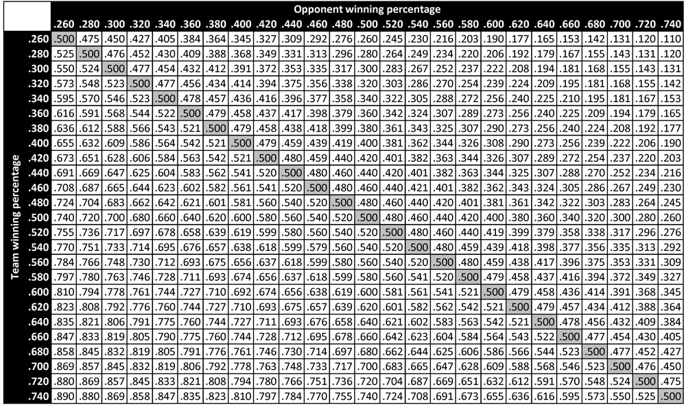
Table 1 (click to enlarge)
Scooped by Bill James
Several trends are apparent in Table 1. First of all, regardless of a team’s winning percentage, its predicted probability of victory uniformly decreases as its opponent’s winning percentage increases. Similarly, given an opponent with fixed winning percentage, this opponent is more likely to be defeated by a team with a higher winning percentage. These trends are, of course, related: because every head-to-head matchup yields exactly one win and one loss, each above-diagonal element of Table 1 is equal to the complement of its corresponding below-diagonal element, and each on-diagonal element is identically .500.
Figure 2 presents a graphical depiction of the predicted probability of victory for teams of various qualities. In particular, this figure plots predicted win probability in head-to-head matchups as a function of opponent winning percentage. This figure contains 11 traces, representing the predicted probabilities of victory for 11 hypothetical teams with winning percentages ranging from .250 to .750 in steps of .050. (The team winning percentage corresponding to each trace is indicated immediately to the left of the trace.) The dashed vertical lines demarcate the same range of opponent winning percentages (.250 to .750) as spanned by the traces.
If the win-probability function P looks familiar, it may be because it first appeared in print over thirty years ago. As is the case for so many sabermetric devices, it was originally proposed by Bill James. In his 1981 Baseball Abstract, James wrote an article entitled “Pythagoras and the Logarithms” in which he proposed this same relationship, albeit on completely different grounds.5 In particular, in contrast to the constructive derivation presented here, James used an essentially axiomatic approach to derive the win-probability function: he stated a set of properties that any sensible win-probability function must possess (such as those indicated above), and then suggested a function that did in fact possess those properties.
James christened his technique the “log5” method. Although apparently originally cast in a different (and more complicated) format, the win-probability relationship was reworked by James and colleague Dallas Adams into the same format constructively derived here. James used this formula repeatedly in later Baseball Abstracts; it has since been used by others in a variety of sabermetric contexts. James and Adams apparently performed a limited behind-the-scenes empirical validation of the log5 method, stating that the selected empirical data “matches very closely” (emphasis in original) with the win-probability function. Unfortunately, details were not provided. In the following section, we provide a detailed quantitative empirical validation of the win-probability function, demonstrating that its predictions are in excellent agreement with historical results.
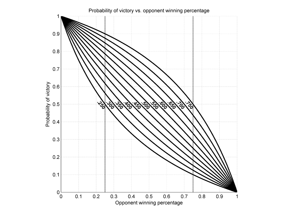
Figure 2 (click to enlarge)
Comparison with Empirical Results
From the inception of the National Association in 1871 through the conclusion of the 2013 season, there were exactly 206,017 regulation regular-season major league baseball games.6 Exactly 204,858 of those games ended in victory for one team, with the other 1,159 games ending in a tie. The 204,858 decisive games comprise an excellent data set for evaluating the validity of the win-probability function.
We will evaluate the accuracy of the win-probability function by comparing its theoretical predictions to empirical head-to-head winning percentages observed between teams of various qualities. In all comparisons, each team’s full-season winning percentage will be used as the measure of its inherent quality, and not its season-to-date winning percentage; the former provides a much better estimate of the true quality of a team, and the latter is far more variable (especially early in a season). In order to facilitate the analysis, interpretation, and presentation of the results, we will group teams into winning-percentage bins with extents of .020. For instance, teams with winning percentages between .490 and .510 will be grouped into a single bin centered at .500 for analysis; similarly, teams with winning percentages between .510 and .530 will be grouped into another bin centered at .520.7 Figure 3 depicts a histogram of team winning percentages throughout major league history, separated into these bins.8
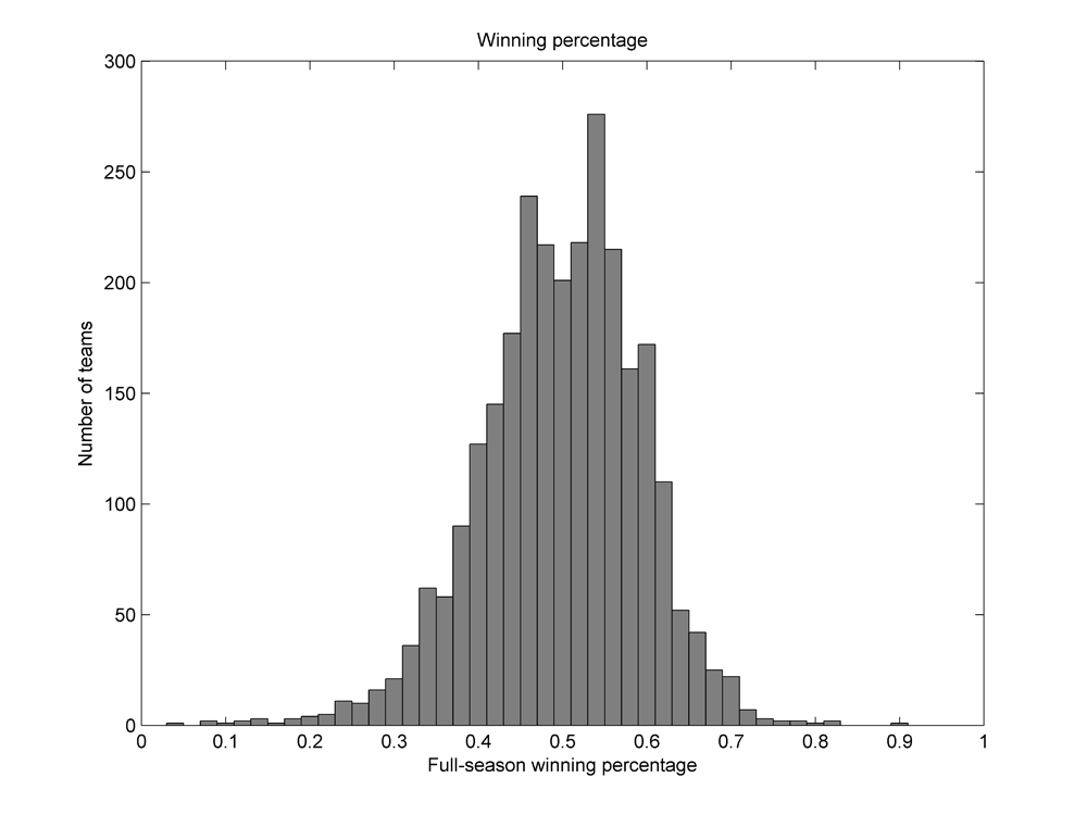
Figure 3 (click to enlarge)
Table 2 presents empirical probabilities of victory in all head-to-head matchups between teams of all qualities for the entirety of major league history.9 Each cell in Table 2 lists the empirical probability of victory for a team with quality (i.e., full-season winning percentage) in the bin indicated by the heading of the corresponding row, when facing a team with quality in the bin indicated by the heading of the corresponding column.10 (Matchups that have never occurred in major league history—for instance, a .280 team facing a .720 opponent—are simply indicated by the absence of a number.) Note that because every head-to-head matchup yields one win and one loss, each above-diagonal element of Table 2 is equal to the complement of its corresponding below-diagonal element, and each on-diagonal element is identically .500.
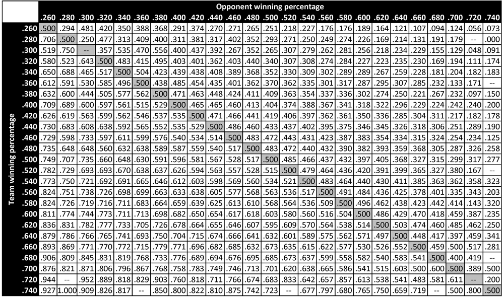
Table 2 (click to enlarge)
We can compare the predicted probabilities of victory in Table 1 to the empirical probabilities of victory in Table 2 to get a sense of the accuracy of the former table’s predictions (and thus the accuracy of the win-probability function P). For example, among all teams in major league history that ended the season with a winning percentage in the .600 bin (that is, between .590 and .610), the empirical probability of victory when facing an opponent with winning percentage in the .400 bin (that is, between .390 and .410) is observed to be .682. In comparison, the predicted probability of victory for a .600 team facing a .400 opponent is .691—a difference of less than 1% in absolute terms. Similarly, when a .600 team faces a .500 opponent (who thus represents a league-average team), its empirical probability of victory is seen to be .603—a very slight deviation from the theoretical value of .600. When a .600 team faces another .600 team, its empirical probability of victory is empirically .500 (a result that follows necessarily from the zero-sum nature of win-loss accounting), which is the same as the predicted value. Finally, when a .600 team faces a .700 opponent, its empirical win probability is .459. This is somewhat larger than the theoretical value of .391 indicated in Table 1; the larger deviation (compared to the others noted here) can be attributed to the relatively rare occurrence of such a matchup and the resulting small sample size. In particular, there have been 1359 decisive matchups between a .600 team and a .400 team, 1815 decisive matchups between a .600 team and a .500 team, and 846 decisive matchups between two .600 teams. In contrast, there have only been 185 decisive matchups between a .600 team and a .700 team. A larger deviation in the empirical probability is thus to be expected. Table 3 presents the number of decisive matchups in major league history between teams of different qualities—that is, the sample size for each of the empirical probabilities in Table 2. Note that Table 3 displays a fundamental symmetry: its above-diagonal elements are identical to the corresponding below-diagonal entries.
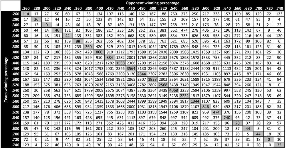
Table 3 (click to enlarge)
The same theoretical trends that were apparent in Table 1 are also apparent in the empirical data of Table 2. As predicted, a team’s empirical probability of victory tends to decrease as its opponent’s winning percentage increases; similarly, an opponent with a fixed winning percentage is generally more likely to be defeated by a team with a higher winning percentage. As with Table 1, each above-diagonal element of Table 2 is equal to the complement of its corresponding below-diagonal element, and each populated on-diagonal element is identically equal to .500.
A cell-by-cell comparison of Table 1 and Table 2 demonstrates that there is, in fact, excellent agreement between the theoretical and empirical probabilities of victory in head-to-head matchups. In particular, there is generally very close agreement between predicted and empirical probabilities in matchups characterized by a large sample size (as indicated in Table 3). The cells for which there are larger mismatches tend to be those with smaller sample sizes, for which empirical variation is inherently fundamentally larger. This suggests that the theoretical predictions provided by the win-probability function P are in fact borne out by actual results over the course of major league history.
We can bring this qualitative, inspection-based assessment of the theoretical predictions and empirical observations onto firmer quantitative ground. In particular, we can apply a metric known as the Brier score11 to quantify the level of agreement between theory and observation. Originally developed to evaluate the accuracy of weather forecasts, the Brier score is more generally used to measure the accuracy or predictive power of a probabilistic assessment over numerous trials. It can be applied whenever probabilities are assigned to a set of mutually exclusive, collectively exhaustive discrete outcomes.12 We will rely on a formulation known as the Brier skill score,13 which essentially represents a comparison of the predictive power of a model to that of a naïve model that assumes that each outcome is equally likely—in this case, a trivial model specifying an equal (.500) probability of victory for each team in any matchup, regardless of the teams’ levels of quality.14 A Brier skill score of 1 indicates perfect predictive power, while a Brier skill score of 0 indicates predictive power limited to that of the naïve uniform-probability benchmark.15 The greatest possible Brier skill score would be achieved by a fully empirical win-probability function—that is, a function E that simply used the empirical probabilities of victory throughout major league history, as presented in Table 2, as a lookup table for its probability estimates.16 We can thus reference the success of the theoretical win-probability function P by comparing its Brier skill score SP to the greatest-possible Brier skill score SE that is achieved by the fully empirical function E. In particular, we will calculate an “efficiency ratio” RP for the win-probability function P:
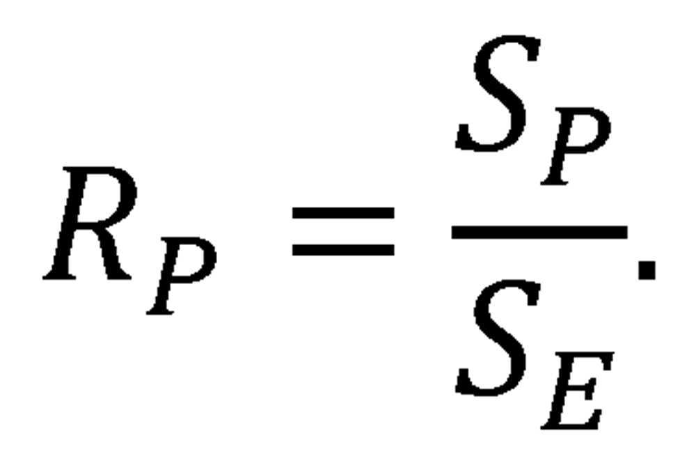
This efficiency ratio provides an unambiguous, absolute measure of the accuracy of the win-probability function P. A ratio of 1 indicates a perfect match between theory and practice, and a value less than 1 indicates an imperfect match (with the degree of imperfection indicated by the deviation from unity).
Table 4 presents the scoring metrics for the theoretical win-probability function P as calculated from the full set of decisive games in major league history. Of primary interest is the efficiency ratio Rp: it is nearly 98%, indicating that the win-probability function has nearly as much predictive power as the empirical data. Clearly, the win-probability function provides an excellent model for the actual probability of victory in head-to-head matchups.
Table 4: Scoring metrics for the theoretical win-probability function
| Brier score (BP) |
Brier skill score (SP) |
Efficiency ratio (RP) |
|---|---|---|
| 0.2361 | 0.0556 | 0.9790 |
In addition to evaluating the accuracy of the win-probability function across the entirety of major league history, we can examine its accuracy across different major league eras. Table 5 presents a somewhat arbitrary—but nevertheless relevant—partitioning of major league history into seven distinct eras, along with the number of decisive games in each era. The empirical win probabilities for head-to-head matchups in each of these seven major league eras, as calculated from the full set of decisive games in each era, are similar in character to the empirical win probabilities for the entirety of major league history. Due to space limitations, the empirical results for each era are not presented in the body of this article, but are instead provided in an online appendix.17
Table 5: Major-league history partitioned by era
| Era | Start | End | Games |
|---|---|---|---|
| Pre-modern | 1871 | 1900 | 20,456 |
| Dead-ball | 1901 | 1919 | 23,700 |
| Live-ball | 1920 | 1946 | 33,067 |
| Integration | 1947 | 1960 | 17,241 |
| Expansion | 1961 | 1976 | 28,184 |
| Free-agency | 1977 | 1996 | 41,081 |
| Interleague | 1997 | 2013 | 41,129 |
We can use the previously introduced scoring metrics to quantify the agreement between theoretical predictions and empirical results in each era. Table 6 presents the Brier score, Brier skill score, and efficiency ratio achieved by the win-probability function P in each of the seven major league eras. This table demonstrates that the fidelity of the win-probability function is excellent—and essentially unchanged—across major league eras. In particular, P achieves an overall efficiency ratio between 90% and 94% in each era, with a mean of 92.04% and a standard deviation among eras of only 1.15%.
Table 6: Scoring metrics for the theoretical win-probability function in different major-league eras
| Era | Brier score (BP) |
Brier skill score (SP) |
Efficiency ratio (RP) |
|---|---|---|---|
| Pre-modern | 0.2182 | 0.1272 | 0.9380 |
| Dead-ball | 0.2315 | 0.0740 | 0.9201 |
| Live-ball | 0.2346 | 0.0617 | 0.9297 |
| Integration | 0.2364 | 0.0544 | 0.9035 |
| Expansion | 0.2400 | 0.0401 | 0.9128 |
| Free-agency | 0.2418 | 0.0330 | 0.9148 |
| Interleague | 0.2405 | 0.0379 | 0.9241 |
The efficiency ratios of Table 6 are all slightly smaller than the 97.90% efficiency ratio observed for the entirety of major league history. This is attributable to the smaller sample sizes—and the resulting greater inherent empirical variability—within individual eras.18 The consistency of the efficiency ratios across eras, however, demonstrates that the predictions of the win-probability function are in excellent agreement with the empirical probabilities of victory in every major league era. In other words, the win-probability function is a valid, high-fidelity model of the actual probabilities of victory in head-to-head matchups regardless of era.
A Slight Revision
We now consider a slight revision to the win-probability function P in an attempt to provide even greater agreement with empirical results. This revision is based on a careful consideration of the interpretation of “league average” in the context of specific teams meeting for a head-to-head matchup.
As stated at the outset of this article, winning percentage is the best statistical indicator of team quality relative to the league in which a team plays. In addition to providing a measurement of team quality, however, winning percentage also provides information about the relative quality of the rest of the league. In particular, if Team A finishes its season with a winning percentage over .500, then we know that the rest of Team A’s league, taken as a whole, has finished the season with a winning percentage under .500. Conversely, if Team A ends the season with a sub-.500 winning percentage, this implies that the rest of the league has an ensemble winning percentage over .500. For an N-team league in which all teams play the same balanced schedule, we can express this relationship exactly: if Team A has a winning percentage of WPA, then the rest of Team A’s league must have a winning percentage of

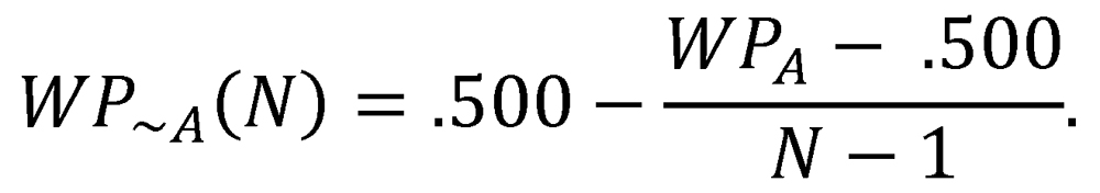
This has interesting implication: from the perspective of an above-.500 team, the league-average opponent is actually below .500, and from the perspective of a below-.500 team, the league-average opponent is actually above .500. An above-.500 team would thus seem to derive some extra benefit from playing its schedule against teams that are somewhat worse than average, while a below-.500 team would seem to compound its woes by playing teams that are somewhat better than average. This points directly to a flaw inherent in the win-probability function: P(WPA,WP~A) actually exceeds WPA for an above-.500 team and falls short of WPA for a sub-.500 team. Clearly this is an absurdity, since a team with winning percentage WPA should, by definition, be expected to post a winning percentage of exactly WPA in the context of its league.
We can modify the form of the win-probability function by adjusting the values of its two arguments, WPA and WPB, to counteract this effect. In particular, if Team A and Team B are both members of the same N-team league, then we can adjust each team’s winning percentage as follows:

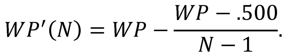
This has the effect of adjusting a team’s winning percentage downward or upward by the same amount by which its opponents’ ensemble winning percentages exceeded or fell short of .500, respectively. We then take the revised win-probability function P’ to be

![]()
This revised function represents an attempt to bring a team’s predicted win probability against a league-average opponent, rather than a league-average team, into agreement with its winning percentage.19
Table 7 presents the probabilities of victory predicted by the revised win-probability function. Comparison to Table 1 (the probabilities of victory predicted by the original win-probability function) reveals that the revised function hedges its bets slightly. In particular, the revised win-probability function judges the outcome of any contest between teams of different qualities to be slightly less certain—that is, to have closer to even odds—than suggested by the original win-probability function.
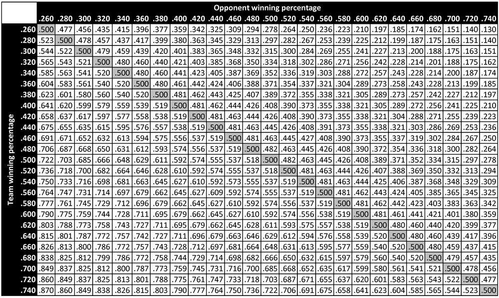
Table 7 (click to enlarge)
As with the original win-probability function, we can compare the predictions of the revised win-probability function with empirical results. Table 8 presents the Brier scores, Brier skill scores, and efficiency ratios for both the original and revised win-probability functions, as calculated for the entirety of major league history.20 The revised win-probability function is seen to attain a slightly higher efficiency ratio (98.32%) than the original win-probability function (97.90%). Although this is an absolute increase of only 0.42%, it represents a 20.2% reduction in the residual error when compared to the empirical upper bound—that is, a reduction of unmodeled empirical variation from 2.10% to 1.68%. As such, it represents a nontrivial improvement in model fidelity.
Table 8: Scoring metrics for the revised and original theoretical win-probability functions
| Function | Brier score (B) |
Brier skill score (S) |
Efficiency ratio (R) |
|---|---|---|---|
| Original (P) | 0.2361 | 0.0556 | 0.9790 |
| Revised (P’) | 0.2360 | 0.0558 | 0.9832 |
Table 9 presents results for the original and revised win-probability functions for the seven previously defined major league eras. It is evident from Table 9 that the revised win-probability function provides greater agreement to empirical results for every major league era except the pre-modern era. (The pre-modern era might be expected to exhibit the most significant deviations from theory given the relatively extreme distribution of team quality, the sometimes haphazard nature of scheduling, and the occasionally irregular league composition that were endemic to the time.) Calculated across the seven eras, the revised win-probability function achieves a mean efficiency ratio of 92.35% (an improvement from the original function’s mean of 92.04%), and exhibits a standard deviation of just 0.81% (an improvement from the original function’s standard deviation of 1.15%). Thus, whether considered over the entirety of major league history or within individual major league eras, the revised win-probability function is seen to provide even better agreement to empirical results than the original function.
Table 9. Scoring metrics for the revised and original theoretical win-probability functions in different major league eras


Table 9 (click to enlarge)
Conclusion
Team winning percentages translate directly to probabilities of victory in head-to-head matchups. The relationship between a team’s winning percentage and its probability of victory when facing an opponent from the same league is shown to be derivable on theoretical grounds; this derivation is straightforward and follows directly from a thought experiment involving the two teams in question and a hypothetical third proxy team. The theoretical win-probability function thus derived is identical to a function proposed on entirely different grounds by Bill James in 1981. The win-probability function is shown to be in excellent agreement with empirical major league results, not only over the entirety of major league history but also within arbitrary major league eras. A slight refinement of the theoretical win-probability function is shown to yield even better agreement with empirical results.
It should be noted that the win-probability function described here can be applied without caveat only to teams in the same league: it does not strictly apply to head-to-head matchups between teams in different leagues with potentially different inherent qualities. Rigorous expression of win probabilities in such cases would require adjustments to account for the relative levels of quality of the distinct leagues in which the teams posted their respective winning percentages. Even so, for matchups between teams from different leagues of essentially equal quality—for instance, the American League and the National League—the win-probability function presented here can be expected to be accurate.
It should also be noted that rigorous application of the win-probability function requires not only that the teams under consideration be members of the same league, but also that they play the same balanced schedule in that league. Major league teams have not played balanced schedules since the advent of divisional play in 1969; schedule imbalance was further exacerbated with the inception of interleague play in 1997. However, Table 6 and Table 9 indicate that unbalanced schedules have not had a notable effect on the accuracy of the win-probability function. Thus, although perfect schedule balance may be a requirement for the theoretical derivation of the win-probability function, mild-to-moderate schedule imbalance does not seem to present an impediment to its practical use.
Although this article has focused exclusively on the probability of victory in head-to-head team matchups, the concepts and methods used here are readily extensible to other contexts involving matchups between entities in which there are two possible outcomes. Most directly, the win-probability function could be applied without significant modification to situations involving distinct binary outcomes in which the league-average probability of success is identically .500—say, contests between starting pitchers.21 Similarly, the framework used here might be modified to express the probabilities of distinct binary outcomes in situations where the league-average probability of success is not identically .500—say, the probability of a batter with a particular batting average getting a hit when facing a pitcher with a particular opponents’ batting average.22 Finally, our framework might be modified to provide the probabilities of various events in situations characterized not by binary outcomes, but rather by a set of several possible outcomes—say, the probability of a particular plate appearance resulting in a strikeout, walk, home run, or ball in play, given the individual propensities of the batter and the pitcher to produce each outcome. Although the required extensions to the current framework may be nontrivial, it is likely that they could be made on similar theoretical grounds as employed here.
JOHN A. RICHARDS first discovered sabermetrics when he picked up a copy of “The Bill James Baseball Abstract 1988.” He was hooked right away. He is an avid Red Sox fan, an affliction he acquired during a decade of college and graduate school in Boston. John is an electrical engineer who has been applying various techniques from his field to sabermetrics for years, but this is his first publication in the “Baseball Research Journal.” He lives in Albuquerque with his wife and son. He was the happiest man in New Mexico on three October nights in 2004, 2007, and 2013.
Acknowledgments
I wish to thank Jacob Pomrenke and Jerry Wachs, each of whom graciously provided me access to resources that were extremely valuable in the composition of this article.
Appendix: https://sabr.org/journal/article/appendix-1-probabilities-of-victory-in-head-to-head-team-matchups/
Notes
1. These rules exhibit the so-called “transitive property” that is sometimes invoked informally in sports arguments (and rather more formally in mathematical proofs).
2. This derivation relies on the assumption that the winning percentages of Team A and Team B are neither both 0 nor both 1. If both teams have winning percentages of 0 or 1, then we can simply take each team’s probability of victory to be .500 (as would in fact be indicated by a straightforward extension of this derivation).
3. As suggested in passing at the beginning of this article, true team quality may be essentially unknowable (or, at least, not measurable to arbitrary precision). However, it is our contention that full-season winning percentage provides the best measurement of true, inherent, unobservable team quality. As such, the term “quality” will be used throughout the remainder of this article to refer to full-season winning percentage.
4. It should be noted that this table, like the others in this article, presents results for a much wider range of team qualities than is typically observed even over the course of multiple seasons. The wide range of qualities serves to illustrate trends and matchups that, while rare, are still historically relevant.
5. Bill James, “Pythagoras and the Logarithms,” 1981 Baseball Abstract (Lawrence, Kansas: self-published, 1981), 104–10.
6. There has been considerable argument and discussion about whether the National Association actually qualifies as a major league. Somewhat arbitrarily, it is treated as a major league here. Game total from Retrosheet game logs, available at www.retrosheet.org.
7. In a 162-game season, the .500 bin encompasses teams that won 80, 81, or 82 games, while the .520 bin encompasses teams that won 83, 84, or 85 games. Although finer distinctions are possible, they are not necessarily statistically meaningful, and they would cloud the presentation of the results.
8. Some of the “noise” apparent in Figure 3—that is, the fluctuation between counts in adjacent bins—is due to the non-constant number of discrete won-lost records that map to each bin in a fixed-length season. For instance, over a 162-game season there are three distinct win totals (80, 81, and 82) that map to the .500 bin, and three distinct win totals (83, 84, and 85) that map to the .520 bin. However, there are four distinct win totals (86, 87, 88, and 89) that map to the .540 bin. This leads to an inflation in the population of some bins that is unavoidable without choosing a bin width equal to an integer multiple of 1/162. (Note also that any bin width enabling population by constant numbers of discrete win totals in a 162-game season would not achieve this result in a 154-game season.)
9. These data were compiled from Retrosheet game logs, available at www.retrosheet.org.
10. For ease of presentation and interpretation, the very small number of teams that ended a season with a winning percentage below .250 or above .750 are aggregated into the .260 and .740 bins, respectively.
11. Glenn W. Brier, “Verification of Forecasts Expressed in Terms of Probability,” Monthly Weather Review, 78 (1), April 15, 1950, 1–3.
12. When applied to a collection of probabilistic predictions and corresponding outcomes over a set of N binary trials (i.e., trials in which only two outcomes are possible), the Brier score takes the form B = ∑ N i = 1 (Pi – oi )2. Here, Pi is the predicted probability of a given outcome in trial i, and oi is an indicator variable that takes value 1 if the given outcome is realized and value 0 otherwise. In our context, Pi is the predicted win probability provided by P, and oi indicates whether victory was actually achieved.
13. Allan H. Murphy, “Skill Scores Based on the Mean Squared Error and their Relationships to the Correlation Coefficient,” Monthly Weather Review, 116 (12), December 1988, 2417–24.
14. The Brier skill score S and the raw Brier score B are related by the equation S = 1 – 4B.
15. A negative Brier skill score is also possible, indicating predictive power worse than that of the naïve uniform-probability benchmark.
16. Such a fully empirical predictor is, in a myopic sense, the highest-fidelity predictor that is possible: its predicted win probabilities exactly match the empirical probabilities in the system it seeks to model. In another sense, however, a fully empirical predictor is highly suspect: its alleged greater fidelity is actually only an encapsulation of specific random instances of statistical variability that fluctuate around a deeper, simpler trend, despite the fact that this variability would be expected to lessen as more and more data became available. Furthermore, the dubious improvement in fidelity achieved by a fully empirical predictor would be achieved only at the cost of a dramatic increase in complexity.
17. This appendix can be found at http://sabr.org/node/32297.
18. This effect is even more pronounced if attention is restricted to even smaller sample sizes, such as individual major league seasons—or, in the extreme, individual series or games. This does not imply that the predicted probabilities of victory are less valid, or that the underlying probabilities of victory are any different, over small samples. It simply reflects the fact that measurements obtained from limited samples are necessarily characterized by greater statistical variability.
19. In fact, this revision does not quite achieve the desired result: because each of the two arguments is adjusted independently, there will still be a slight discrepancy between P’(WPA,WP~A,N ) and WPA (albeit much smaller than the discrepancy of the original win-probability function) whenever WPA is not .500. Additional modification of the win-probability function might enable further reduction in the size of this discrepancy, but only at the cost of the introduction of significantly more complexity. Such modifications are not pursued here.
20. The results in Table 8 and Table 9 were calculated using representative values of league size N for each era. In particular, N = 8 was used for the pre-modern, dead-ball, live-ball, and integration eras; N = 11 was used for the expansion era; N = 13 was used for the free-agency era; N = 15 was used for the interleague era. The value N = 12 was used for the entirety of major league history.
21. In this case, the possibility of a no-decision would either need to be explicitly disallowed, or the framework would need to be modified to accommodate this possibility.
22. As with the previous case, the possibility of a nondecisive outcome such as a base on balls would either need to be explicitly disallowed, or the framework would need to be explicitly modified to accommodate it.