What Baseball Team Does PageRank Say Was the Best Ever?
This article was written by Gwen Ostergren - Michael Krebs
This article was published in Spring 2022 Baseball Research Journal
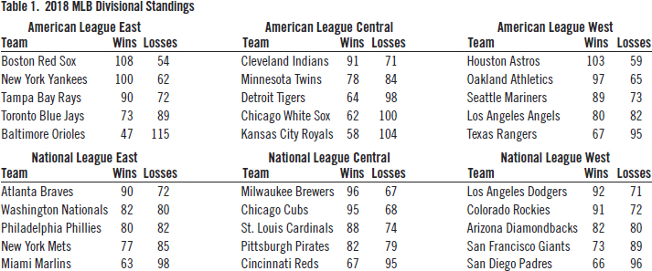
Charles Dickens may well have written about baseball’s American League East in 2018 that it was the best of teams, it was the worst of teams. This grouping of only one-sixth of all Major League Baseball (MLB) clubs contained both baseball’s winningest team that season (the Boston Red Sox, 108 wins) as well as its losingest (the Baltimore Orioles, 47 wins). Nearest to Boston was the Houston Astros with 103 wins, and behind them, the New York Yankees with 100. Baltimore’s nearest competitor for fewest wins was the Kansas City Royals with 58, and the Chicago White Sox finished third-to-last in this category with 62 wins. Neither the Astros, White Sox, nor Royals belong to the American League East division. With rare exceptions, every team plays exactly 162 games each season. (The Brewers in 2018 were one of those rare exceptions, playing 163, but this has a negligible impact on our analysis.)
(Click image to enlarge)
Table 1 shows the regular-season win-loss record for all MLB teams in 2018. Based on this evidence alone, baseball aficionados could conclude that the Red Sox were a better team than any other in 2018, and that every other team was better than the Orioles. Most players would also surely agree that their objective each season is to win as many games as possible, as each division winner advances to the playoffs.
The 30 MLB teams are grouped into two “leagues” (American and National), and each league is grouped into three divisions (East, Central, and West). Each team plays only 20 interleague games, and only against select opponents. For example, in 2018 the Atlanta Braves (NL) faced the Tampa Bay Rays (AL) only four times, and they did not play any games at all against the Los Angeles Angels (AL). Moreover, each team will play others in the same division more frequently than those in other divisions. For example, the NL West’s Arizona Diamondbacks played 19 games against division-mates the San Diego Padres, but only six versus the NL East Philadelphia Phillies. The Orioles and Red Sox took each other on 19 times, and the Red Sox emerged victorious on 16 of those occasions.
The mere fact that Baltimore and Boston went up against one another so often casts doubt on the assertion that Boston was the best and Baltimore was the worst in 2018. Surely the Red Sox benefited from having a weak team like the Orioles to beat up on with disproportionate frequency. Conversely, did not the Baltimore Orioles suffer for having to contend so often with the likes of the Red Sox?
In 2018, the Chicago White Sox beat the Red Sox four times. They also beat the Orioles four times. MLB’s standard accounting method treats those eight wins equally. Somehow, though, we would like to weight the four victories over Boston, a strong team, more heavily than the four victories over the Orioles, a weak team. More generally, we wish to weight each win according to the prowess of the defeated team. How can we assign these weights?
THE PageRank ALGORITHM
The PageRank algorithm provides one method for determining these weights. Consider, for example, only three teams from 2018: the Orioles, the Red Sox, and the White Sox. Let x1, x2, and x3 be values assigned to those three teams, respectively. Our goal is to determine x1, x2, and x3.
The Orioles had 16 losses in 2018 to the Red Sox and 4 to the White Sox, for a total of 20 against those two teams. Also, the White Sox had 3 losses each to the Red Sox and to the Orioles. So, 4/5 of the Orioles’ losses and 1/2 of the White Sox’s losses (against the teams under consideration) were to the Red Sox. PageRank then assigns a weight to the Red Sox by taking 4/5 of the Orioles’ weight plus 1/2 of the White Sox’s weight. That is:
We can interpret this equation as follows. Each victory over the Orioles contributes x1/20 to the value of x2, and each victory over the White Sox contributes x3/6.
In the same vein, we obtain two more equations for the other two teams. We can consolidate this system of equations into the following matrix equation:
Solving, we find that every solution is a multiple of x1 = 50, x2 = 63, and x3 = 46.
Observe that because these values assigned by PageRank reflect the team’s strength, we thereby obtain a new way to rank teams: in order of PageRank values. In our example, then, first place goes to the Red Sox (score of 63), second place to the Orioles (50), and third place to the White Sox (46).
We can view equation (1) as saying that (x1, x2, x3)T is an eigenvector with eigenvalue 1 for the given matrix. More generally, given any collection of n teams, let A be the matrix whose (i,j) entry equals the number of times team i defeated team j divided by the total number of losses suffered by team j. (We ignore the possiblity that a team may be undefeated—this has never happened in major-league history.) Then we find the corresponding PageRank values x1,…,xn by requiring that (x1,x2,…,xn)T is an eigenvector for A with eigenvalue 1. We can uniquely determine the xi by additionally requiring that x1 +•••+ xn =1.
One may well ask whether 1 is always an eigenvalue for A, and if so, if the corresponding eigenspace always has a single basis vector with only positive entries, as in our example. As to the first question, the answer is yes. That’s because, by construction, the columns of A sum to 1. Consequently, vA = v, where v= (1,1,…,1). Taking transpose of both sides, we get that ATvT = vT, so vT is an eigenvector for AT with eigenvalue 1. The result follows, as a matrix and its transpose have the same eigenvalues.
The second question is a bit deeper, but equally crucial. Without one-dimensionality, PageRank will not produce a unique ranking of teams. Even in the case that the eigenspace is one-dimensional, if a basis vector v for it contains both positive and negative entries, we will not know whether to use v or – v for our solution. Choosing – v instead of v will reverse the rankings. Fortunately, the Perron-Frobenius theorem answers this question by providing conditions under which things work the way we want. We will not discuss this theorem further here—see, for example, C.R. MacCluer’s work for more about it1—but rest assured that throughout this paper, whenever we use PageRank, these conditions are met, so our rankings are indeed well-defined.
Originally, PageRank was developed not to rank sports teams, but so the Internet search engine Google could rank websites.2 In this application, websites take the place of baseball teams, and one website does not defeat another, but rather is pointed to by a hyperlink from it. To deal with issues such as “islands” of websites which cannot access other parts of the Internet via hyperlinks, one typically introduces a damping factor, as we shall discuss later.
In the case of Internet searches, the values xi have an intuitive meaning. First we limit ourselves to a collection of websites related to a given search term, say, those that contain this term or are linked to by a page containing it. We then imagine a “random web surfer” who begins by selecting one of these websites at random. Our Internet addict then randomly picks one of the links on that page and follows it. The process continues ad infinitum. The value xi equals the limit, as the number of steps goes to infinity, of the probability that the surfer will be at website i.
Many publications have previously discussed the use of PageRank to rate sports teams.3 Moreover, as discussed there and elsewhere, there are many other rating and ranking systems, including Elo, PowerRank, Pythagorean expectation, and more.
NPR: NORMALIZED PAGERANKS
We applied the PageRank method to the 2018 MLB season—and lo and behold!—the Astros, not the Red Sox, emerged as the top-rated team. Moreover, the Kansas City Royals had the lowest PageRank score, despite the Orioles having eleven fewer wins. Why? Perhaps because the Houston Astros play in the AL West, which overall seems to have been a tougher division. While Houston had fewer wins than Boston, those wins were on average weighted more heavily, enough for PageRank to crown the Astros best in baseball in 2018. On the other end of the spectrum, the Royals play in the AL Central, a notably weak division whose best team in 2018 (Cleveland) was ranked by PageRank as 20th out of 30 MLB teams.
PageRank also ranked the Chicago White Sox above the Detroit Tigers and the Philadelphia Phillies above the Washington Nationals, even though the Tigers had more wins than the White Sox and the Nationals had more wins than the Phillies.
We now apply this method to every baseball season beginning, somewhat arbitrarily, in the year 1900. Our analysis includes all teams 1900 through 2018. If we assign PageRank scores x1,x2,…,x30 to the 30 2018 MLB teams while imposing the condition that x1 + x2 +•••+x30=1, then the average PageRank score will be 1/30. In 1918, however, there were only 16 teams (eight in each league), so the average for that year would be 1/16, nearly twice as high as the average score a century later. Simply doing a head-to-head comparison would give the earlier teams an unwarranted edge.
Even worse, teams from different leagues did not face one another prior to 1997. So the American League and National League form separate “islands,” in which case the Perron-Frobenius theorem will no longer guarantee a unique solution. From 1900 to 1996, we therefore apply PageRank separately to the two leagues. But then in 1918, for example, the average score would be 1/8.
To compare between years and leagues, then, we define the Normalized PageRank (NPR) as the number of sample standard deviations the PageRank score is above the sample mean of PageRank scores of teams within a comparison group. From 1900 to 1996, the comparison group is the set of all teams in the same year and in the same league. From 1997 to 2018, the comparison group is the set of all teams in the same year.
In 2018, we expect the Astros and Red Sox to have a positive NPR (they were almost certainly better-than-average teams) and the Royals’ and Orioles’ NPRs to be negative (below average). This is indeed the case. The 2018 Houston Astros had an NPR of 1.324, just barely edging out the Boston Red Sox, with their NPR of 1.316. The Kansas City Royals had an NPR of -2.079, worse than the Baltimore Orioles’ -1.948.
SOME ADDITIONAL NOTES
When interpreting a t-statistic such as NPR, it is useful to confirm that the underlying distribution is normal. For this purpose, we created Q-Q plots (not shown here). Based on these, we are confident that the PageRank scores are normal, and we may therefore interpret the NPR scores accordingly.
Unlike soccer, where games frequently end in ties, baseball teams generally play until one is victorious. However, it is rare but not impossible for an MLB game to end in a tie. This can happen, for example, when a game ends early due to weather conditions and is late enough in the season that it is not subsequently completed. In fact, more than one thousand MLB games have ended without a winner. When computing NPR scores, we disregarded these games. We also considered only the American and National Leagues. We did not analyze the short-lived Federal League, for example.
The 2012 Cincinnati Reds are an interesting case study. They won 3/5 of their games and had a winning percentage of 0.599. (To refer to this as a winning “percentage” is a standard misnomer in baseball; it simply means number of wins divided by number of games played.) By this measure, they were a much better than average team. However, their NPR was – 0.02. So PageRank regards them as a below-average team, albeit just slightly. How can this be? In the National League that year, only the Braves and Nationals had positive NPRs. PageRank seems to have determined on the basis of the interleague games that year that the AL on balance was considerably better than the NL that year.
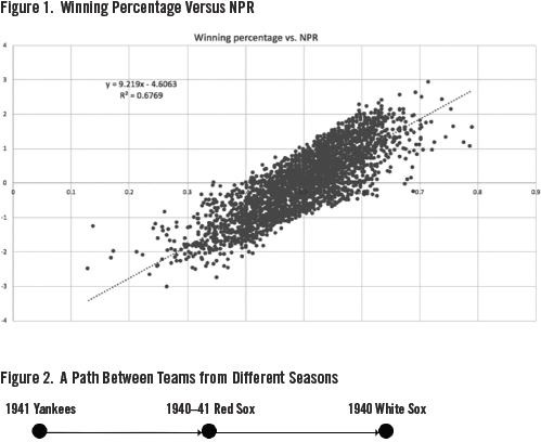
In general, though, NPR correlates positively with winning percentage, as one would expect. We can see this in Figure 1, which shows a scatterplot of winning percentage versus NPR. We performed a simple linear regression and found that r2 = 0.6769.
(Click image to enlarge)
NPR2: COMPARING TEAMS ACROSS YEARS
In the procedure described in the previous sections, we effectively formed a directed multigraph by representing each team in a given season as a vertex, and representing each game as a directed edge from the loser to the winner. Let G be the (undirected) multigraph obtained by disregarding orientation of edges. The resulting graph is highly disconnected. Indeed, each connected component of G corresponds uniquely with either a season since 1997 (when interleague play started) or with a league and a season prior to 1997.
One can easily find a path, for example, from the 2018 Atlanta Braves to the 2018 Los Angeles Angels. Although those two teams never faced one another directly, the 2018 Braves did play the 2018 Tampa Bay Rays, who in turn played the 2018 Angels. But no path exists between teams from different seasons. Nor can one find a path between an American League team and a National League team prior to 1997, as teams then played only other teams in the same league.
NPR, therefore, does not account for variation in average team strength from season to season, or from league to league pre-1997. During World War II for example, many players, including several superstars, took a hiatus from baseball to serve in the armed forces. The first players were inducted into the military in 1941. It is plausible, therefore, that although the 1940 Chicago White Sox and the 1941 Boston Red Sox had roughly equal NPRs (1.032 and 1.045, respectively), the former team was stronger. Likewise, expansion years, when the major leagues added teams, may have diluted the talent pool. The year 1962, which introduced new teams in Houston and New York, exemplifies this phenomenon. The 1962 New York Mets have an NPR of -2.406, the 10th lowest out of the 2,504 teams in our database.
In an attempt to address this issue, we now add several new vertices and edges to our directed graph. Each new vertex will represent not a team in a single season but rather a team over the span of two seasons. For each game, we add directed edges from the loser to the winner, where both endpoints represent one-year or two-year teams. We chose to insist, however, that at least one of the two endpoints should be a one-year team. For example, then, a game in 1940 in which the White Sox beat the Red Sox would show up as five edges in our new graph:
- an edge from the 1940 Red Sox to the 1940 White Sox
- an edge from the 1940-41 Red Sox to the 1940 White Sox
- an edge from the 1940 Red Sox to the 1940-41 White Sox
- an edge from the 1939-40 Red Sox to the 1940 White Sox
- an edge from the 1940 Red Sox to the 1939-40 White Sox
Continuing this example, we additionally factor in a game in 1941 in which the Red Sox beat the Yankees. For now let’s consider only that outcome together with the aforementioned 1940 White Sox victory over Boston. Within our graph, then, we will have a path from the 1941 Yankees to the 1940 White Sox, as shown in Figure 2.
This path has the effect of giving the 1940 White Sox “points” for beating a team that beat the 1941 Yankees. In this way we can account for “strength of schedule” across seasons—or even, by taking longer and longer paths, across eras.
We include a vertex for a two-year team only when the team existed both years. We have no vertex for the 1961—62 New York Mets, for example, as the Mets were founded in 1962.
The two-year vertices serve as bridges from one season to the next. Consequently, in our new graph, there is a path from any one-year team to any other one-year team. In the case of teams in different leagues before 1996, one must take a somewhat circuitous route, first making one’s way to 1997, then switching leagues via an interleague game. Given a directed multigraph, the PageRank method produces a matrix A with 1 as an eigenvalue, as described in Section 2. Using this new, connected graph, PageRank provides a means for comparing teams in different seasons.
We applied the PageRank method to this matrix A but found the results to be unsatisfactory. In the results, the top 100 teams were all in the National League. That seems unrealistic. We speculate that PageRank may have found the National League in 1997 to be stronger on average than the American League that year, and due to the structure of our graph, this deficit may have been impossible to overcome. In other words, although the two-year teams eliminate islands, the graph is still fairly “clumpy.”
Fortunately, we have a standard technique to deal with this situation. Namely, we introduce a damping factor α, where α is a value between 0 and 1. Let B be a square matrix of the same size as A. Let C=(1 – α)A + αB. We then find a positive-valued eigenvector for C with eigenvalue 1 and assign scores to teams accordingly.
The damping factor takes a small portion of the score assigned to each node and redistributes them evenly throughout the graph, thereby mitigating the clumpiness. In the random web surfer model, we can view a as the probability that the user does not follow a link from the current page, but rather simply selects an Internet page at random to visit next.
We took α=0.15 as our damping factor, as this is a standard, frequently used value. As with NPR, we then normalize by computing the number of sample standard deviations above the sample mean. We call the resulting value the team’s NPR2 score. The “2” refers to the inclusion of two-year teams.
Because the NPR2 eliminates islands, we use the set of all teams from all years when computing mean and standard deviation. By contrast, with NPR, we calculated separately for separate comparison groups.
(Click image to enlarge)
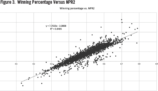
As with NPR, we also have that NPR2 correlates positively with winning percentage. Figure 3 shows a scatterplot of winning percentage versus NPR2. We performed a simple linear regression and found that r2=0.8527. So NPR2 correlates more closely with winning percentage than does NPR. This may be partly due to the damping factor we included with NPR2. It may also be partly because, with regression to the mean, we would anticipate less of a spread in the weights attached to victories for two-year teams than for single-year teams.
A JUSTIFICATION FOR THE METHOD
Adding nodes for two-year teams makes little sense unless a team’s performance one year correlates with its performance the following year. Intuitively, we expect that it should, as teams usually retain most of their players from year to year. We consider it a good habit to back up intuition with data, however.
Towards this end, we used a permutation test to compare the mean absolute difference between a team’s winning percentage one year and its winning percentage the following year against the absolute difference between a team’s winning percentage and a randomly selected other team. Our specific procedure went as follows. Between 1900 and 2017, we identified 2,506 teams that continued to exist the following year. Let w1,…,w2506 be the winning percentages of these 2,506 teams, and let u1,…,u2506 be the respective winning percentages of these teams the following year. For example, our first team under consideration is the 1900 Brooklyn Superbas. So the Superbas’ winning percentage in 1900 is w1 » 0.603, and their winning percentage in 1901 is u1 » 0.581. We then take the absolute differences \w1-u1\,…,\w2506– U25o6\. The sample mean m of these 2,506 absolute differences is approximately 0.060. In other words, on average, a team’s winning percentage changes by about 6 percentage points from one year to the next.
We claim that this is a smaller change than one would expect by choosing two teams randomly. To test this claim, using Mathematica, we randomly selected a set P of one hundred elements from S2506, the symmetric group on 2,506 letters. For each element  , we calculate the mean mj of the absolute differences
  . Taking the set
  as our sample, we find that the sample mean is about 0.095, and the sample standard deviation is about 0.001.
So m is approximately 34.6 standard deviations below the mean of the mj. A Q-Q plot (not depicted here) shows the mj to be distributed approximately normally. We may therefore state with confidence that a team’s winning percentage one year is far closer to its winning percentage the following year than one would expect due to randomness alone.
RESULTS
So far, we have discussed three scores we can assign to a given team in a given year: winning percentage, NPR, and NPR2. We may briefly describe these three rating systems as follows. Winning percentage gives the fraction of games won. NPR describes how much better or worse than average a team fared, taking into account the strength of its opposition that season. NPR2 does the same as NPR, but also considers the opponents’ strength across a two-year period.
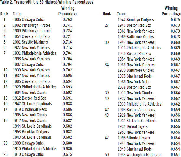
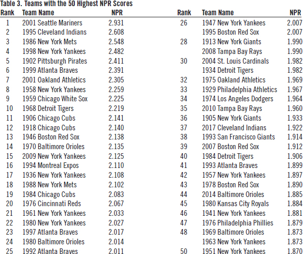
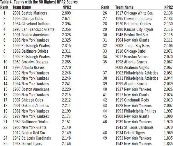
Tables 2, 3, and 4 show the top 50 modern-era MLB teams with respect to these scores. Note that the same team has both the highest NPR and the highest NPR2 score ever: The 2001 Seattle Mariners. For that reason, we regard the 2001 Seattle Mariners as the answer to this paper’s title question.
In fact, only three teams appear amongst the top 10 in all three lists, namely, the 1902 Pirates, the 2001 Seattle Mariners, and the 1998 New York Yankees.
Many consider the 1927 Yankees to have been the best team ever. Neither NPR nor NPR2 agrees with this assessment, however. Despite having the sixth-best winning percentage since 1900, they rank 21st by NPR2 and only 19th by NPR.
(Click images to enlarge)
POSSIBLE VARIATIONS
There are innumerable ways to vary the techniques discussed in this paper, and we make no claim that our choices were optimal. In this section, we mention a few, but by no means all, potential alternative paths.
We chose to count all victories equally. We could have taken the margin of victory (that is, runs scored minus runs allowed) into account. It would be interesting to know how that would affect the results.
We also opted to use only regular-season games. We excluded all postseason games, including the World Series. Because World Series games are played between one AL and one NL team, this would have provided a bridge between leagues, even before interleague play.
For NPR2, we added two-year teams, but we just as easily could have added three-year teams, four-year teams, and so on. For that matter, instead of having additional nodes that encompassed entire seasons, each added vertex could instead represent a team during the last half of one season and the first half of the next season.
PageRank, of course, is only one of many methods that account for “strength of schedule.” We like it because of its mathematical elegance. The main novel idea of this paper—namely the introduction of two-year teams in order to compare across eras—can however be used with other such techniques as well.
MICHAEL KREBS conducted this research while at California State University, Los Angeles, where he has been a professor of mathematics since 2005.
GWEN OSTERGREN has previously collaborated on projects in pure mathematics (more specifically, geometric graph theory) with Michael Krebs at California State University, Los Angeles. Collectively, they have published several articles in that field.
Acknowledgments
The authors would like to thank Jie Zhong for a helpful discussion. We would also like to thank Mike Freiman for informing us about the websites Baseball-Reference.com and Retrosheet, from which we collected all of the data used in this paper. In addition, we are grateful to the anonymous reviewers of our original manuscript; their many thoughtful comments substantially improved the final product. Moreover, we thank the Baseball Research Journal’s eagle-eyed fact checker Cliff Blau for spotting numerous errors and affording us the opportunity to correct them.
Notes
1. C.R. MacCluer, “The many proofs and applications of Perron’s theorem,” SIAM Review 42 (3), 2000, 487-498.
2. Sergey Brin and Lawrence Page, “The anatomy of a large-scale hypertextual web search engine,” Computer Networks and ISDN Systems, Vol. 30 (1-7), April 1998, 107-17.
3. Previous investigations of PageRank in sports include T.PE. Chartier, E. Kreutzer, A. N. Langville, and K. E. Pedings, “Sensitivity and stability of ranking vectors,” SIAMJ Sci. Comput. 33(3), 1077-102; A.Y. Govan, “Ranking theory with application to popular sports,” Thesis (PhD 2008) North Carolina State University; L.R. Zack, R. Lamb, and S. Ball (2012). “An application of Google’s PageRank to NFL rankings,” Involve 5(4), 463-71.

