

Seven Degrees of Separation? Analyzing MLB Played-With Relationships, 1930-2016
This article was written by Peter Uelkes
This article was published in Spring 2018 Baseball Research Journal
INTRODUCTION
This article reports on MLB “played-with” relationships for the time period 1930 through 2016. We define player A as having played-with player B if the two appeared in the same major league game for the same team. This doesn’t necessarily mean both players stood on the field at the same time. We also include cases where one player had already left the game when the other player entered.
This analysis uses event files as provided by Retrosheet.1 These contain information on starting players as well as in-game substitutions. For most years prior to 1930, only starting players are available, so the analysis only goes back to the 1930 season. By processing the event files, a graph was built containing 13,298 players as nodes (vertices) and 831,835 played-with relationships as edges. We are then able to extend the played-with relationships by including paths from player A to player B via intermediate players.
To quantify this, we define the distance between players A and B as follows:
- distance(A, B) = 0: A player has distance 0 only to himself (A=B)
- distance(A, B) = 1: Players A and B played-with each other as defined above
- distance(A, B) = 2: Player A didn’t play-with player B, but there exists (at least one) player C who played-with A and played-with B (in different games)
- And so on. For example, for distance(A, B) = 3: Player A didn’t play-with player B, and there is no single player C who played-with both players A and B (in different games), but there exists (at least one) pair of players C and D, who played-with each other and one of whom played-with player A, the other with player B. In other words, there is a chain of three played-with steps to get from player A to player B.
In the next step, distances for each pair of players were calculated using a standard algorithm from graph theory known as the Floyd-Warshall algorithm.2 The purpose of this algorithm is to find the shortest path for each pair of nodes (vertices) in a graph. The length of the shortest path then gives the distance measure for each pair of players as defined above. The running time of the algorithm is proportional to the third power of the number of nodes (number of players in our case). There are faster algorithms for finding the shortest path between a specific pair of players or for one specific player to all others, but for this analysis, we need the distance measure for every pair of players, so Floyd-Warshall is the appropriate algorithm.
After running the algorithm on the data set, a number of interesting results can be extracted from the graph and its associated distances.
MAXIMUM DISTANCE
As a first result, we report the distribution of player-player distances for the complete data set as Figure 1.

Figure 1: Histogram of the distance between any two players in the data set. The x-axis represents the distance while the y-axis shows the respective relative frequency. Distance is as defined in the main text.
(Click on any figure image to enlarge.)
The histogram shows a value of three as the most common distance (i.e. as mode of the distribution). The maximum distance is seven. It’s a remarkable result: For any pair of major league players in the time period 1930-2016, we are able to construct a played-with path of no more than seven. There is no pair of players that isn’t connected via a played-with path!
Typically, a maximum-length path includes as one endpoint a player with very few major league appearances, a Moonlight Graham-type career. For example, one such path is:
- Owen Kahn played-with Rabbit Maranville for the Boston Braves vs. the Brooklyn Dodgers on May 24, 1930.
- Rabbit Maranville played-with Danny MacFayden for the Boston Braves vs. the Cincinnati Reds on June 17, 1935 (second game of doubleheader).
- Danny MacFayden played-with Mickey Vernon for the Washington Nationals vs. the Philadelphia Athletics on May 11, 1941.
- Mickey Vernon played-with Harmon Killebrew for the Washington Nationals vs. the New York Yankees on September 20, 1955 (second game of doubleheader).
- Harmon Killebrew played-with Jamie Quirk for the Kansas City Royals at the Texas Rangers on September 26, 1975.
- Jamie Quirk played-with Steve Finley for the Baltimore Orioles at the Toronto Blue Jays on September 29, 1989.
- Steve Finley played-with Robb Quinlan for the Los Angeles Angels of Anaheim at the New York Mets on June 12, 2005.
So the path from Owen Kahn to Robb Quinlan includes six intermediate players, two of whom (Killebrew and Maranville) are in the Hall of Fame. Of course, typically there are several or even many other paths of the same length between two endpoints, in this case, Kahn and Quinlan. Also, it should be noted that Hall of Famers typically have long careers (22 and 23 years for Killebrew and Maranville, respectively), so they play with a lot of other players and therefore act as “hubs” in the network of played-with connections. This is especially the case if they switched teams repeatedly. Maranville, as a case in point, played for five different teams in his career—including the Boston Braves, whom he left after the 1920 season and returned to in 1929.
To further illustrate the difference between Hall of Famers and the bulk of other players, we show as Figure 2 a modified version of Figure 1. This time the data of Figure 1—all player pairs—are shown as black bars while pairs of players who are both in the Hall are shown as dark gray bars. Pairs in which at least one player is in the Hall are represented by light gray bars.
We clearly see that the distribution of pairs of players who were both Hall of Famers (“Both HoF”) is leaning to the left, toward lower distances, compared to the “All players” distribution. The weighted average distance between all players is 3.38, while for pairs of Hall of Famers it’s 2.67. Hall of Famers have smaller average distances than the mean of all players.
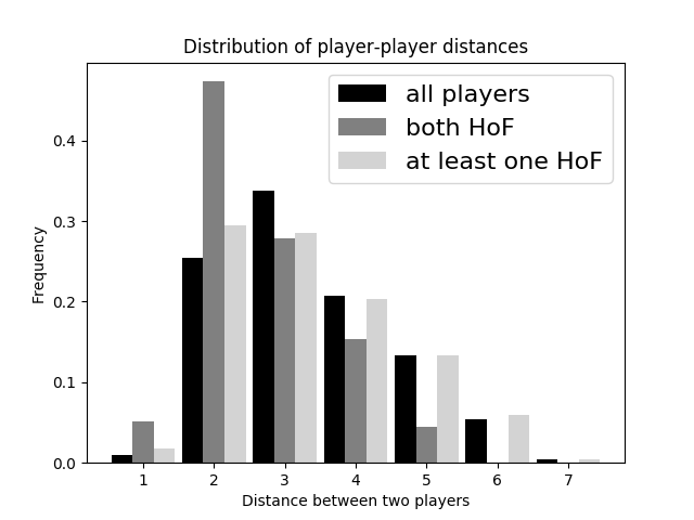
Figure 2: Distribution of the distance between any two players in the data set. The x-axis represents the distance while the y-axis shows the respective relative frequency. Distance is as defined in the main text. Black bars represent all player pairs, dark gray bars represent pairs where both players are in the Hall of Fame (inducted as “Players” as defined at Baseball-Reference.com) and light gray bars represent pairs where at least one player is in the Hall.
Returning to the length-7-path shown above, Robb Quinlan appeared in a fair number of major league games (458). Owen Kahn, on the other hand, appeared in only one. He entered the game on May 24, 1930, as a pinch-runner, scored his run, and never played in the major leagues again.
DIRECT CO-PLAYERS
We define a direct co-player for player A as any player who has a distance of one to player A, i.e. who played-withplayer A. First, we’ll have a look at the overall distribution of the number of co-players per player. We restrict ourselves to players who debuted between 1930 and 2006 (instead of 2016) to eliminate noise from the partial-career data of the many players active in 2016 who debuted in the last decade.
Figure 3 shows a histogram of the number of co-players for each player.
We see a large peak for numbers of co-players below 100. The reason for that is the large number of players who only had a “cup of coffee” in the major leagues and therefore only had a relatively small number of co-players.
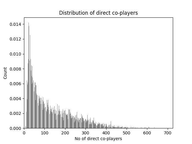
Figure 3: Histogram of the total number of co-players in a career for each player in the data set. The x-axis gives the number of direct co-players (i.e. players with distance = 1) while the y-axis shows the count of how often that number of co-players occurs in the data set.
The highest entry is at 671 co-players (equivalent to about 27 full 25-man rosters). This entry belongs to Rickey Henderson, an inner-circle Hall of Famer who played in the majors for 25 seasons for nine different teams—including four separate stints with one of them, the Oakland A’s. A few other players in the data set have in excess of 600 co-players: Matt Stairs, Terry Mulholland, Carlos Beltran, David Weathers, and LaTroy Hawkins. None of these players is active anymore (Beltran retired following the 2017 season), so none of them will match Rickey-being-Rickey.
At the low end of the distribution is a single player with only eight direct co-players in his career—eight being the minimum possible number. He is Whitey Ock, who played only one game. Owen Kahn, who was mentioned in the previous section for having a distance of seven from Robb Quinlan, has 11 direct co-players from his lone big-league game. A relatively modern player near the low end is Bob Davidson, who played in one game in 1989, with 12 co-players.
Because of the expansion of the major leagues starting in the 1960s and greater mobility of players in the wake of free agency, there is reason to expect a trend of an increasing number of co-players with time. To make that explicit, we look at the mean number of co-players as a function of the debut season of the player in question. See Figure 4.
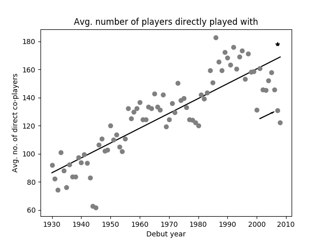
Figure 4: Mean number of direct co-players for a player who debuted in a specific year. The x-axis shows the debut year while the y-axis gives the mean (average) value of direct co-players, i.e. players with distance equal to one, for each player with that debut year. A regression line is shown that is fitted to the data points. The arrow indicates the uncorrected data point for the 2007 debut year while the asterisk shows the corresponding corrected data point. See main text for more information.
We see a clear upward trend, though with some season-to-season fluctuations. This is to be expected as the number of teams has grown via expansion. In addition, a sharp increase is seen in the 1980s with free agency coming into full effect, and therefore much greater mobility of players across teams. Also, a pronounced decline is visible during World War II, when rosters were much more stable than usual. Whether a stabilization takes place in the 2000s is not yet clear because many players from that period haven’t finished their careers.
In order to get a handle on this, an analysis was done taking into account all Hall of Famers (inducted as “Players” as defined at Baseball-Reference.com) who debuted between 1930 and 1989 (so their complete careers are covered by the available data).3 It was then calculated how the number of their direct co-players evolved with the Hall of Famers’ respective age. Figure 5 shows some results for Hall of Famers debuting in four different decades.
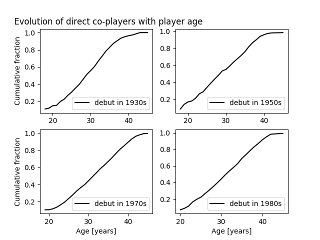
Figure 5: Time evolution of the fraction of direct co-players as a function of the player’s age for Hall of Famers (elected as “Players”) who debuted in a given decade: 1930s (upper left panel), 1950s (upper right), 1970s (lower left) and 1980s (lower right). The x-axis shows the players’ age in years, the y-axis represents the fraction of direct co-players the player ended up with at the time of his retirement who had already directly played with him at that age.
Figure 5 shows evolutions that are close to linear for the age bracket between about 20 and 40 years, i.e. the main part of a player’s career (few players play beyond age 40). It’s therefore, as a first approximation, possible to extrapolate the number of direct co-players for a given player age for an active player. A caveat applies here because the analysis represented in figure 5 was restricted to Hall of Famers (because of technical limitations, Retrosheet does not provide player birth year data, so the analysis software had to be extended to automatically fetch birth years from Baseball-Reference.com) and, of course, not all current players will end up in the Hall.
Keeping this in mind, an exemplary correction was done for players who debuted in 2007. For them, 10 years of major league playing time was represented by the available data set. If they didn’t play in 2016, they were assumed to be retired (introducing a possible small error for players who weren’t retired but missed 2016 because of injury). If they were still active in 2016 and at most 40 years old, their number of direct-co players accumulated by then was corrected by an age-dependent factor that was taken from the lower right panel of figure 5. For example, if the player was 37 years old in 2016, his number of direct co-players was divided by 0.785, because that’s the fraction taken from the Hall of Famer analysis shown in figure 5.
Without this correction, the mean number of direct co-players for players debuting in 2007 was about 131 (see figure 4, data point indicated by arrow). With the correction, the number is about 178, which is closer to the regression line in figure 4 (see data point accompanied by an asterisk). This indicates, taking the rough correction into account, that the trend of an increasing number of co-players is still unbroken in recent years. Because the correction was done based on Hall of Famers’ careers, a certain overcorrection was to be expected because Hall of Famers typically have long careers.
HUBS AND OUTSIDERS
For every player, we took the mean value (average) of the distances to all other players in the data set. Let’s then define players with a large mean distance as outsidersand players with an especially small mean distance as hubs. So outsiders are players who are relatively isolated on the outskirts of the player connection graphs, while hubs are players who are central to the graph, with many other players “close by.”
The top 10 outsiders are:
| Name | Debut year | Mean distance | Co-players |
|---|---|---|---|
| Owen Kahn | 1930 | 5.168 | 11 |
| Johnny Scalzi | 1931 | 4.931 | 22 |
| Walter Murphy | 1931 | 4.903 | 15 |
| Al Wright | 1933 | 4.901 | 21 |
| Bill Dreesen | 1931 | 4.899 | 28 |
| Gordon McNaughton | 1932 | 4.894 | 20 |
| Eddie Hunter | 1933 | 4.885 | 11 |
| Jim Spotts | 1930 | 4.871 | 21 |
| Buz Phillips | 1930 | 4.863 | 29 |
| Monk Sherlock | 1930 | 4.861 | 29 |
These players all are situated at the early end of the data set, which automatically generates a relatively large distance to the (many) modern players. We’ve encountered Owen Kahn, who has the largest mean distance, already as one endpoint of a path with a distance of seven.
Now let’s look at the top 10 hubs:
| Name | Debut year | Mean distance | Co-players |
|---|---|---|---|
| Harold Baines | 1980 | 2.439 | 546 |
| Rich Gossage | 1972 | 2.459 | 504 |
| Julio Franco | 1982 | 2.51 | 579 |
| Jesse Orosco | 1979 | 2.512 | 587 |
| Phil Niekro | 1964 | 2.519 | 369 |
| Rickey Henderson | 1979 | 2.53 | 671 |
| Brian Downing | 1973 | 2.532 | 360 |
| Dennis Martinez | 1976 | 2.533 | 354 |
| Dave Winfield | 1973 | 2.533 | 471 |
| Rick Dempsey | 1969 | 2.539 | 394 |
This table shows players with debut years between 1964 and 1982, during a period when major league baseball was expanding and free agency was coming into being. Even if we look at the 50 smallest mean distances, the most recent debut year is 1983 (Otis Nixon). For more modern players, the distance to the 1930-era players gets too large, bringing up the mean. In a sense, Harold Baines (22 years of service, five teams, including three separate stints with two of them) is the “best-connected” player in the data set.
VISUALIZATION
Once a player-connection graph is built, it is possible to visualize it by using a tool like Gephi.4 Of course, visualizing a graph with more than 13,000 nodes and more than 800,000 edges is a hopeless task. To make this tractable we created graphs for two particular seasons, 1951 and 2004. See Figure 6.
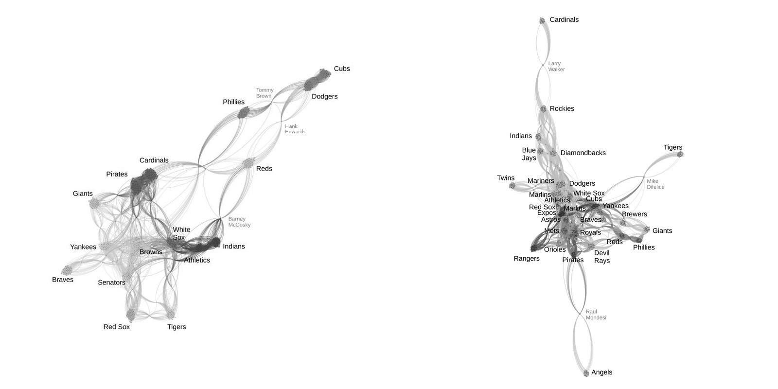
Figure 6: Player connection graphs considering only games played in the 1951 (left panel) or 2004 (right panel) season. Players are shown as small dots while edges of the connection graph are shown as curve segments connecting the dots. The closer that players are clustered together, the smaller the distance between them. Teams are indicated, and their players are, of course, clustered together. A player switching teams midseason (player names in a paler font), like Larry Walker in the 2004 graph, will connect two team clusters.
To create the visualization, the graph was loaded into the Gephi tool. The tool uses a “force atlas” method to create node-to-node distances.5 Also, a modularity analysis was done and nodes were shadedaccordingly. We annotated the generated image with team names.
In a paler font we annotated a few individual player’s names. These are players who switched teams during the season and therefore connect the clusters of nodes (players) for different teams. These examples are, for the 1951 season:
- Barney McCosky was purchased by the Cincinnati Reds from the Philadelphia Athletics on May 4, 1951.
- Hank Edwards was selected off waivers by the Cincinnati Reds from the Brooklyn Dodgers on July 21, 1951.
- Tommy Brown was traded by the Brooklyn Dodgers to the Philadelphia Phillies on June 8, 1951.
Two (or more) teams get clustered close together by the tool if there are strong, i.e. multiple, connections between them. One example is the Dodgers and Cubs, who exchanged multiple players via trade during the 1951 season. Another example is the 1951 Browns, who were involved in multiple player exchanges with several teams and so are right in the middle of the clustering.
The graph for the 2004 season looks more complex than the 1951 graph because there were more major league teams and players in the later season.
In the 2004 graph, we clearly see three teams that are only connected via one player to the bulk of the other teams:
- St. Louis Cardinals (acquired Larry Walker from the Rockies)
- Detroit Tigers (traded Mike Difelice to the Cubs)
- Anaheim Angels (signed Raul Mondesi as a free agent after he was released by the Pirates)
In general, the 2004 player connection graph is more “crowded” than the 1951 graph because of the higher mobility of players, i.e. more player exchanges between teams. This leads to relatively small played-with distances between numerous pairs of teams. In the end, more than half of the teams from the 2004 season are clustered so close together that it’s barely possible to resolve them in the visualization.
So the visualization tool gives us a lot of insight into who played with whom and which teams were connected via in-season player exchanges.
As a further example, we show the connection graph for Hall of Fame players.
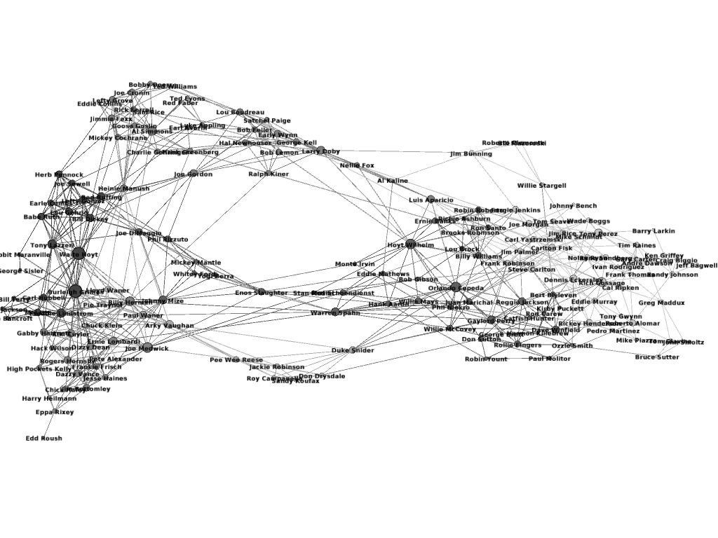
Figure 7: Player connection graph for Hall of Famers, i.e. players who were inducted as “Players” into the Hall of Fame.
We see some clustering, which stems from teams with multiple Hall of Famers. For example, the Los Angeles Dodgers of the 1960s at bottom center, with Sandy Koufax, Don Drysdale, Duke Snider et al. Also, there is a timeline-like component to the graph, with modern players such as Greg Maddux, Jeff Bagwell, and Tim Raines on the right and old-timers on the left.
The graph, even restricted only to Hall of Famers, is still quite crowded. So as a final illustration, the graph for Hall of Fame pitchers only is presented as Figure 8.
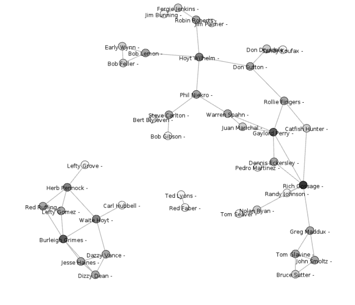
Figure 8: Player connection graph for Hall of Fame pitchers. Please note that Gephi draws connecting lines only for a certain threshold of “closeness,” meaning that, for example, Ted Lyons and Red Faber were not really isolated from the rest of the Hall of Fame pitchers.
SUMMARY
We presented a novel approach to analyzing major league player connections as defined in the played-with sense. In this way, we were able to track historical developments that impacted the structure of on-field personnel, such as expansion and free agency. By using appropriate tools, we presented intuitive visualizations of player connections for selected subsets of the data.
It would be interesting to extend the analysis back in time if more detailed game data (including in-game substitutions) became available for seasons prior to 1930.
PETER UELKES has been a SABR member since 2001. He’s from Germany and became an overseas member of Red Sox Nation in 1990. After receiving a Ph.D in physics, he worked in the finance and telco industries. Living with his wife and their two sons in Germany, Peter spends his time on topics like MLB, soccer, cryptography, astronomy, mathematics, and education.
Notes
1 www.retrosheet.org. The information used here was obtained free of charge from and is copyrighted by Retrosheet.
2 http://en.wikipedia.org/wiki/Floyd–Warshall_algorithm
3 www.baseball-reference.com/awards/hof.shtml
4 Bastian M., Heymann S., Jacomy M. (2009). Gephi: An open source software for exploring and manipulating networks. International AAAI Conference on Weblogs and Social Media.