Actual Pennant Winners Versus Pythagorean Pennant Winners, 1901–2020

This paper will provide a general comparison of actual pennant winners and Pythagorean pennant winners for the National and American Leagues from 1901 to 2020. In part, this is a presentation of data, but it is also an exercise in what might have been. With Pythagorean pennant winners, many teams that did not reach the World Series would have done so. And some Hall of Famers who never played in a World Series would have had the opportunity to do so. Additionally, this paper will include a discussion of luck versus skill in the comparison of actual and Pythagorean pennant winners. All of the data presented herein derive from data on Baseball-Reference.com.

Various terms, such as the Pythagorean Theorem of Baseball (used by Baseball-Reference.com) or the Pythagorean Expectation (used in the Wikipedia article), have been used to describe the formula developed by Bill James in his Baseball Abstract annual volumes to predict the number of games a team “should” have won in a season based on the numbers of runs scored and runs allowed. The formula used currently by Base- ball Reference may be expressed as:

WP=1/{1 + (OR/R)1.83  }

where WP is the predicted winning proportion (i.e., wins divided by the sum of wins and losses), OR is opponents’ runs, and R is runs.

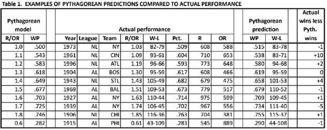
While Pythagorean predictions are shown widely, including on the Baseball Reference website and in the sabermetric literature, I have never come across an illustration showing how OR/R and WP are related, including quantifying the relationship of a change in R/OR with a change in predicted WP. In this regard, successive increases of 0.1 in R/OR starting from 1.0 are associated with declining increases in WP. For example, as R/OR increases from 1.0 to 1.1, predicted WP increases from .500 to .543, or by .043; and as R/OR increases from 1.7 to 1.8, predicted WP increases from .725 to .746, or by .021. The relationship between R/OR and actual and predicted WP is shown in Table 1, comparing modeled values of R/OR ranging from 1.0 to 1.8 and actual values of R/OR for pennant- winning teams ranging from about 1.0 to about 1.8. An R/OR value of 0.6 is included also to provide an example of how the formula applies to a very weak team.

In most cases shown in Table 1, the Pythagorean prediction of WP is very close to the actual winning proportion, and by extension, the Pythagorean prediction of team wins is usually very close (perhaps within three) to actual team wins. There are occasional outliers, illustrated here by Cincinnati in 1961, which won 10 more games than its Pythagorean prediction. Even though the Pythagorean predictions are usually highly accurate, the closeness of many pennant races, with the winning margin often being no more than three games, means that there have been many pennant races in which the actual winner and the Pythagorean winner have been different. In addition, outliers like that Cincinnati team add to the number of cases where the actual and Pythagorean winners have differed. And lastly, the introduction of division play in 1969, with postseason playoffs to determine pennant winners, has decreased greatly the probability of the Pythagorean pennant winner being the actual pennant winner.

 

(Click image to enlarge)

 

OVERVIEW OF ACTUAL AND PYTHAGOREAN PENNANT WINNERS

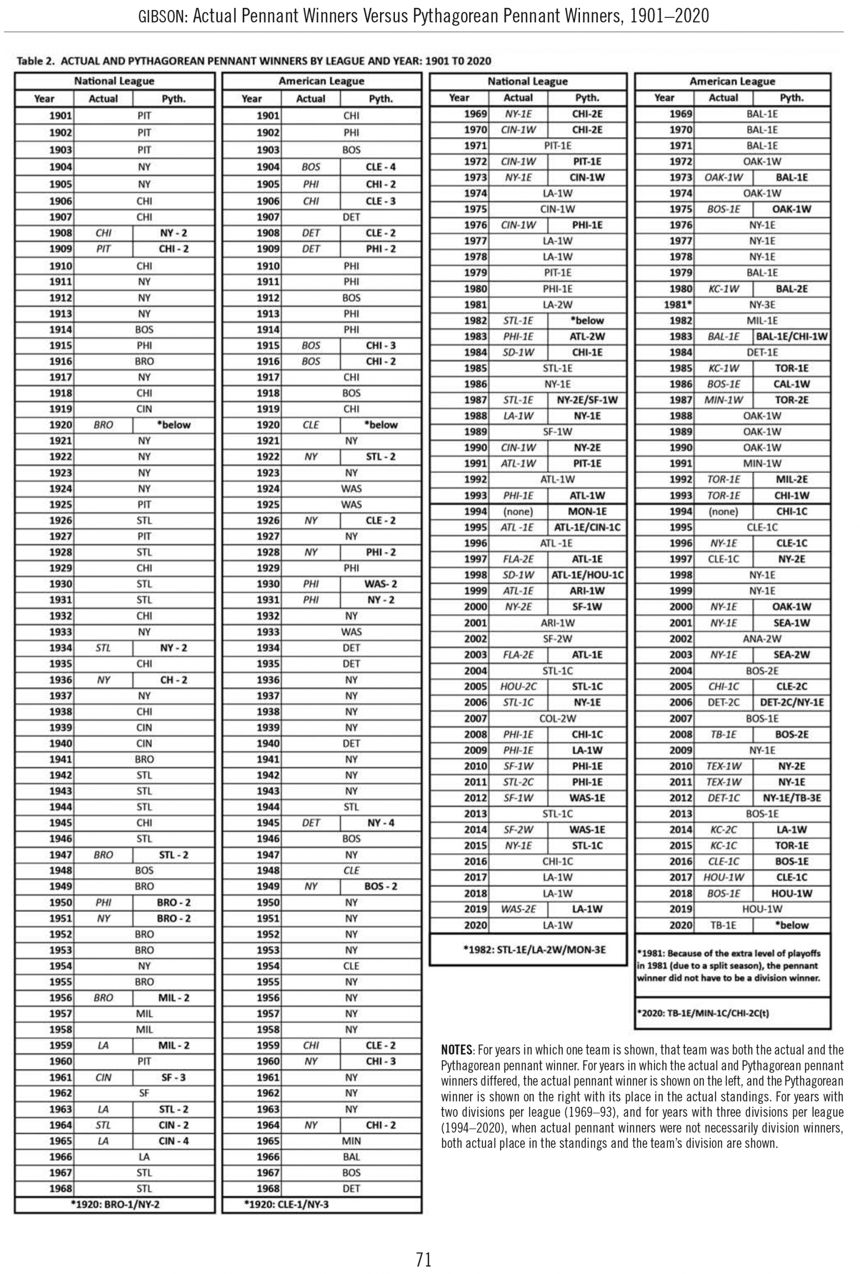
The actual and Pythagorean pennant winners for each season in the National and American Leagues from 1901 to 2020 are shown in Table 2. Calculations of Pythagorean won-lost records were rounded to whole numbers of wins and losses (reflecting the fact that actual won-lost records do not have fractions), and thus there are a few cases with ties for the Pythagorean pennant winner. From 1901 to 1968, before the introduction of division play, the actual pennant winner was also the Pythagorean pennant winner in the large majority of seasons.

A few notable differences in the history of actual and Pythagorean pennant winners are noted here. The Chicago Cubs won four pennants in five years from 1906 to 1910, and won the Pythagorean pennant in 1909, even though the great Pittsburgh Pirates team (110–42) won that actual pennant. The Brooklyn Dodgers, who won six pennants in the 10 years from 1947 to 1956, won six Pythagorean pennants in that decade, including five consecutive ones from 1949 to 1953. The Milwaukee Braves, who won pennants in 1957 and 1958, won four consecutive Pythagorean pennants from 1956 to 1959. And the Cincinnati Reds, who won one actual pennant in the 1960s (1961) won two subsequent Pythagorean pennants (1964 and 1965).

In the American League, the Cleveland Indians, who did not win an actual pennant until 1920, won three Pythagorean pennants in five years: 1904, 1906, and 1908. Three of their great players during those years, Hall of Famers Nap Lajoie, Addie Joss, and Elmer Flick, never played in a World Series. The Detroit Tigers, who won three consecutive pennants from 1907 to 1909, won the Pythagorean pennant in only the first of these three years. The Boston Red Sox won the pennant in 1915 and 1916, but the Chicago White Sox won the Pythagorean pennant in both seasons. Thus Boston won only two Pythagorean pennants from 1912 to 1918 (compared with four actual pennants), and Chicago won four Pythagorean pennants from 1915 to 1919 (compared with only two actual pennants). The St. Louis Browns, who won their only actual pennant in 1944, won the 1922 Pythagorean pennant with the best team in their history, led by Hall of Famer George Sisler, who also never got to play in a World Series.

The New York Yankees and Philadelphia Athletics, loaded with Hall of Fame players, dominated the American League from 1926 to 1931, with three pennants for the Yankees followed by three pennants for the Athletics. The Pythagorean pennant winners for those six years present a different picture: Cleveland (1926), New York (1927), Philadelphia (1928 and 1929), Washington (1930), and New York again (1931). The Yankees dominated the American League with 14 pennants in the 16 years from 1949 to 1964, but won “only” 11 Pythagorean pennants during those 16 years, with Boston (1949) and Chicago (1960 and 1964) also winning Pythagorean pennants.

From 1901 to 1968, there were 136 total seasons of National and American League play. These included 104 seasons in which the actual pennant winner was also the Pythagorean pennant winner, two seasons with a tie for the Pythagorean pennant, and 30 seasons (22 percent) in which the Pythagorean winner differed from the actual winner.

As noted earlier, the introduction of division play and postseason playoffs starting in 1969 changed things dramatically. From 1969 to 1993, with two divisions per league (East and West), there was one tier of playoffs to determine pennant winners. Since 1995, with three divisions per league (East, Central, and West), there have been two tiers of playoffs. (There was no postseason in 1994.) And since 2012, there has been a wild-card game before the two tiers of playoffs to determine pennant winners. In contrast to the 1901 to 1968 period, when the Pythagorean winner was also the actual winner a large majority of the time, since 1969 the Pythagorean winner has had to survive an increasing number of short postseason series to be the actual winner as well.

As a result, there are fewer cases of repeat winners since 1969, with only three cases of a team winning three consecutive actual pennants and Pythagorean pennants, all in the American League: Baltimore, 1969 to 1971; New York, 1976 to 1978; and Oakland, 1988 to 1990. Among the many cases of teams winning the Pythagorean pennant, but not the actual pennant, are the Chicago Cubs (1969 and 1970) and the Seattle Mariners (2001 and 2003). As a result Hall of Famers Ernie Banks and Edgar Martinez, and likely future Hall of Famer Ichiro Suzuki never had the opportunity to play in a World Series.

 

(Click image to enlarge)

 

During the 1969 to 1993 period, there were 50 total seasons of National and American League play. These included 28 seasons in which the actual pennant winner was also the Pythagorean pennant winner, three seasons with a tie for the Pythagorean pennant, and 19 seasons (38 percent) in which the Pythagorean winner differed from the actual winner. From 1995 to 2020, there were 52 total seasons of play. These included 19 seasons in which the actual winner was also the Pythagorean winner, five seasons with a tie for the Pythagorean pennant, and 28 seasons (54 percent) in which the Pythagorean winner differed from the actual winner. Thus seasons in which the Pythagorean winner differed from the actual winner increased from 22 percent before divisional play to 38 percent when there were two divisions and to 54 percent in the cur- rent three-division-plus-wild-card period.

LARGEST DIFFERENCES BETWEEN ACTUAL AND PYTHAGOREAN PENNANT WINNERS

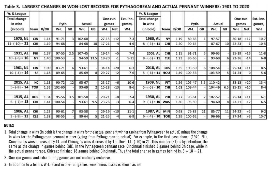
The most interesting seasons in my opinion are those in which there was the greatest total change in the won-loss records of the actual and the Pythagorean pennant winners, the leading case being the 1970 National League. Chicago won the Pythagorean pennant by three games over Cincinnati (94–68 versus 91–71). Cincinnati, which won the postseason playoff to win the pennant, had a 102–60 record compared with 84–78 for Chicago. Thus there is a 21-game difference in the actual and Pythagorean won-loss records of these two teams.

The second largest change involves the great Philadelphia Athletics team of 1931, with a 107–45 won- lost record (and a winning average of .704), which won the pennant by 13.5 games. They outperformed their Pythagorean prediction by 10 games while the New York Yankees, the Pythagorean pennant winner, underperformed by six games.

Data for the 12 seasons with a total change of 10 or more games in going from the Pythagorean pennant winner to the actual pennant winner are shown in Table 3. Seasons with a tie for the Pythagorean pennant are excluded. As in Table 2, the actual pennant winner is listed first; however, the data shown in Table 3 start with the R/OR ratio and the corresponding Pythagorean won-lost record, then show the actual won-lost record to show how the season evolved compared with the Pythagorean prediction. Data are shown also on the team’s actual record in one-run games and extra-inning games, which may shed light on the change from predicted to actual performance.

It should be noted that with postseason playoffs starting in 1969, the actual pennant winner may have been outclassed in both its actual and Pythagorean won-lost records. One example of this is the 1987 American League season, when Minnesota, a very average team during the season (R/OR=0.98) won the American League pennant in postseason play. Toronto had a much better Pythagorean won-lost record than Minnesota (100–62 versus 79–83), and both Detroit (98–64) and Toronto (96–66) had much better actual won-lost records than did Minnesota (85–77).

What accounts for the large changes shown in Table 3? Not surprisingly, teams that had a better actual won-lost record tended to do well in one-run games, and teams that had a better Pythagorean record tended not to do as well in such contests. (Data shown on extra-inning games are not discussed here because such records are subject to more random variation due to being fewer in number.) In the first season in the table, 1970 in the National League, the differences were pronounced. Cincinnati had a 27–15 record in one-run games (12 games over .500), while Chicago had a 17–21 record (four games below .500). Among the 12 seasons shown in Table 3, the differences ranged from pronounced to no appreciable difference. An ex- ample of the latter is provided by the 1987 American League season discussed above. The won-lost records in one-run games were nearly identical for Minnesota (24–22) and Toronto (27–24).

 

(Click image to enlarge)

 

It would be expected that differences in performance in games decided by more than one run also could account for some of the differences noted between actual and Pythagorean records. In this regard, data on games by margin of victory are shown below for Cincinnati and Chicago in 1970. Not only did Cincinnati do better in one-run games than Chicago (27–15 versus 17–21), but also in two-run games (22–9 versus 9–19), three-run games (17–10 versus 15–12), four-run games (14–5 versus 10–9), and five-run games (8–1 versus 7–8). Chicago did better only in games decided by six or more runs (26–9 versus 14–20). Among games decided by five or fewer runs (the large majority of games), the won-lost records were 88–40 for Cincinnati and 58–69 for Chicago. Cincinnati’s nickname—the Big Red Machine—gained prominence in 1970 when the team won 70 of its first 100 games. Perhaps “winner of close games” would have been more accurate, since Chicago scored more runs during the season than Cincinnati (806 versus 775).

LUCK AND SKILL

There has been a lot of research in recent decades on the role of luck in how well a team performs over the course of a season. The Baseball Reference website, in its tables showing detailed standings by season, includes each team’s actual and Pythagorean records and labels the difference between them as “luck,” and quantifies it as actual games won minus Pythagorean games won. Bill James, in his 2004 article “Underestimating the Fog” (BRJ, Vol. 33, pages 29–33) said that with regard to the assertion that winning or losing close games is luck: “it would be my opinion that it is probably not all luck,” suggesting that it was mostly luck. Examples of research focused on the role of luck over the course of a season include Phil Birnbaum in his 2005 article, “Which Great Teams Were Just Lucky?” and Pete Palmer in his 2017 article, “Calculating Skill and Luck in Major League Baseball.”1

Both Birnbaum and Palmer stress the fact that, for an average team with an 81–81 record, one standard deviation corresponds to 6.36 wins, calculated as the square root of (162 x .5 x .5). Rounding one standard deviation to the nearest whole number (six) means that an average team’s record would range from about 75–87 to about 87–75 about 68 percent of the time (reflecting the proportion of the area under a bell-shaped curve within one standard deviation of the mean). Two standard deviations correspond to 12.72 wins. Rounding two standard deviations to the nearest whole number (13) means that an average team’s record would range from about 68–94 to about 94–68 about 95 percent of the time (reflecting the proportion of the area under a bell-shaped curve within two standard deviations of the mean). Thus about five percent of the time, an average team’s record for a season would be 94–68 or even better, or 68–94 or even worse! (These results are identical to those for the results of flipping a fair coin 162 times, expressed as the numbers of heads and tails.) 

While a team with an 87–75 record might have been viewed traditionally as slightly above average and a team with a 94–68 record might have been viewed traditionally as a good team, the reality is not so simple because random variation plays a major role in a team’s performance for a season. For example, a comparison of two teams, one with a 100–62 won-lost record and the other with a 90–72 record yields the following. Their standard deviations in wins are 6.19 and 6.32, respectively. The standard error of the difference between these two values, calculated as the square root of (6.19 squared +6.32 squared) is 8.85. The difference in wins between the two teams (10) divided by the standard error of the difference (8.85) is about 1.13, frequently referred to as the z-score. A z-score of 1 or more means that there is a 68 percent chance that the 100-win team is actually better than the 90-win team. A z-score of 1.13 corresponds to a 74 percent chance. A z-score of 2.0 would correspond to a 95 percent chance that the 100-win team is better. It is a matter of judgment what z-score value is used and depends how much the researcher wants to avoid concluding that the 100-win team is truly superior when this is not the case. However, it is most prudent (as in the case of most medical research) to use the more rigorous standard: a z-score of 2.0 or more corresponding to a 95-percent-plus confidence level before concluding that the difference in records was not due entirely to luck.

It has seldom been the case that the actual and Pythagorean pennant winners differed in wins by nine or more (corresponding generally to one standard deviation or more) and never by as much as 18 or more (two standard deviations or more). The largest difference was in the 1987 American League when, as discussed earlier, the difference between Minnesota’s actual pennant-winning record and Toronto’s Pythagorean pennant-winning record was 15 wins. It may be noted that it is also extremely rare that the “best team” (not necessarily the actual or Pythagorean pennant winner) in a season can be determined. This is because a season (with “only” 162 games) does not provide a large enough sample size to conclude that a team is the best team in its league unless it wins 18 or more games than any of its opponents.

It should be stressed, however, that the Pythagorean pennant winners are the result of a statistical model. A team’s record is determined by the aggregate performance of its players (batting, base running, fielding, and pitching). But this is a two-stage process. Player performance determines, subject to some variation, the numbers of runs scored and runs allowed by the team, which in turn determines the team’s won-lost record. In each of these two phases, a team can under-perform, perform as predicted, or over- perform. All the calculations above, starting with the 6.36 standard error for an average team’s won-lost record, reflect these two phases. The Pythagorean pennant winners are predicted with a model that starts with the team’s numbers of runs scored and runs allowed, thus excluding the variation inherent in an actual baseball season. Thus it may be the case that standard errors calculated for Pythagorean pennant winners should be different (and somewhat lower) than for actual pennant winners. It is my guess that it would still be the case that only a small proportion of the seasons with different actual and Pythagorean pennant winners would differ by one standard deviation or more in their records and that seasons with differences of two standard deviations or more would be extremely rare (perhaps just the 1987 American League).

SUMMARY

The purpose of this paper has been to provide a general comparison of actual pennant winners and Pythagorean pennant winners for the National and American Leagues from 1901 to 2020. From 1901 to 1968, before the introduction of postseason play to determine pennant winners, the actual and Pythagorean pennant winners differed only 22 percent of the time in 136 seasons of play. The corresponding figure for the 50 seasons of play in the 1969 to 1993 period, with one round of playoffs to determine pennant winners, was 38 percent. For the 1995 to 2020 period, with two or more rounds of playoffs to determine pennant winners, the corresponding figure for the 52 seasons of play was 54 percent. There have been 12 seasons with different actual and Pythagorean pennant winners in which the total change in actual and Pythagorean won-lost records was 10 or more games. The most extreme case was in the National League in 1970 when Chicago won the Pythagorean pennant by 3 games over Cincinnati, but Cincinnati actually won 18 more games than Chicago did, a net change of 21 games. Finally, it appears that for all or virtually all seasons in which the actual and Pythagorean pennant winners differed, the differences between the two teams’ won- lost records fell within the range of sampling error on their won-lost records (using a 95-percent confidence level) and thus could be attributed to luck.

CAMPBELL GIBSON, PhD, is a retired Census Bureau demographer, with interests in baseball ranging from biography to statistical analysis. His first article in the Baseball Research Journal was “Simon Nicholls: Gentleman, Farmer, Ballplayer” published in Vol. 18 (1989). His article “WAA vs. WAR: Which is the Better Measure for Overall Performance in MLB, Wins Above Average or Wins Above Replacement?” was published in Vol. 48, No. 2 (2019).

 

Acknowledgments

The author would like to acknowledge the comments and suggestions of two anonymous reviewers.

 

Notes

1. Phil Birnbaum, “Which Great Teams Were Just Lucky?” Baseball Research Journal, Volume 34 (2005): 60–68; Pete Palmer, “Calculating Skill and Luck in Major League Baseball,” Baseball Research Journal, Volume 46, 1 (2017): 56–60).