Another Look at Runs Created

One of the many things that make baseball great is the ability to both objectively and subjectively compare which players are the best. These comparisons range anywhere from scholarly research1 to radio talk show discussions to barroom arguments.

In comparing players, many times researchers have developed new statistics in an attempt to find one all-encompassing number and more objectively assess the value of one player versus other players of their eras. This number can then be adjusted to league averages and for park effects to compare players of all eras. Nowadays, the number most often used in this vein is OPS (On-Base Percentage plus Slugging Average, also known as Production).

This measure is popular mainly because it is a “simple but elegant measure of batting prowess, in that the weaknesses of one-half of the formulation, On-Base Percentage, are countered by the strengths of the other, Slugging Average, and vice versa.”

Another such statistic, Runs Created (RC) was developed by Bill James, based upon the fact that the “best hitter is the hitter who creates the most runs.”3 Over the years James has introduced several more complicated versions of the RC formula, each adding more statistics not available in all eras (e.g., hit-by­ pitch), to more closely associate the value to runs.4

However, one of the disadvantages of developing a single number is that you lose the component numbers and traditional statistics, which are, arguably, more fun to compare. At the same time, comparing players of different eras is quite difficult using many of these component statistics, simply because many are next to impossible to adjust due to such large differences in league averages over the years.5

In his New Historical Baseball Abstract, Bill James created two algorithms for adjusting these component statistics using his RC formula. In his Willie Davis comment (pp. 740-43), James used the first algorithm for adjusting Davis’ statistics as if each of the teams he was on had scored 750 runs per year.6 In his Sam Crawford comment (pp. 795-96), James expands on the first algorithm by including a second algorithm to convert Crawford’s Deadball Era statistics as if he had started his career in 1920 instead of 1900.7 Rather than using a constant 750 runs per year, James used what­ ever amount the team Crawford was on in a particular year had scored 20 years later.

Using the Sean Lahman Baseball Archive Database (v. 5.0) available online at www.baseball1.com, and Microsoft Access Basic/SQL, I created a hybrid of James’s two algorithms to adjust all player statistics (1876-2002) as if their teams had scored 750 runs per year, as well as adjusting for the Deadball Era conver­sion, and park factors. By adjusting for each of these factors, we can then better compare players’ traditional statistics across eras and teams.

Methodology

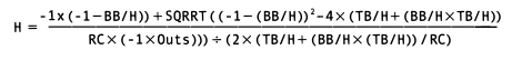
As in James’ algorithms, all counting batting statistics rise and fall with hits. Therefore, the RC formula is adjusted as the elements relate to hits. Thus, the formula becomes:

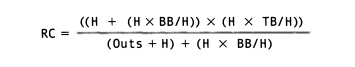
From there, you solve the equation for H. Without going into the algebra to make the quadratic equations that result, the formula to solve for H is:

For each season prior to 1920, the program first converted the appropriate statistics using James’ 1920 algorithm. Then, for each season the program converted the RC based upon the players’ team scoring 750 runs,8 adjusting for park factors.9 The adjusted runs created (RC_ADJ) were then substituted into the hits formula above, using the old ratios (with the conver­sions for pre-1920, where appropriate) for all other elements in the formula. This then gives us H_ADJ.

The ratio between H_ADJ and H was then used to compute BB_ADJ, TB_ADJ, and most other counting statistics. The ratio between RCADJ and RC was then used to compute R_ADJ, and RBI_ADJ. As with James’s algorithms, games played, batting outs (AB – H) and strikeouts remained the same.

Discussion

Not surprisingly, the players with the most change were the pre-1920 players, due to the Deadball Era algorithm (especially players in the early years of baseball, who because teams of that era scored so many runs, had their statistics decrease dramatically — except home runs, of course, which due to the Deadball Era algorithm still rose greatly).

Of post-1920 players, the players most affected on the negative side were not surprisingly, players of the 1920s. On the positive side, also not surprisingly, players of the 1940s-1950s and 1960s-1970s were most affected.

The players of today were not so greatly affected (except for park effects) because, except for a few exceptions in recent years, average runs per team in the leagues have been close to 750 runs per year. In addition, players who have played for longer have had any big league-wide run-producing years offset by lower league-wide run-producing years.

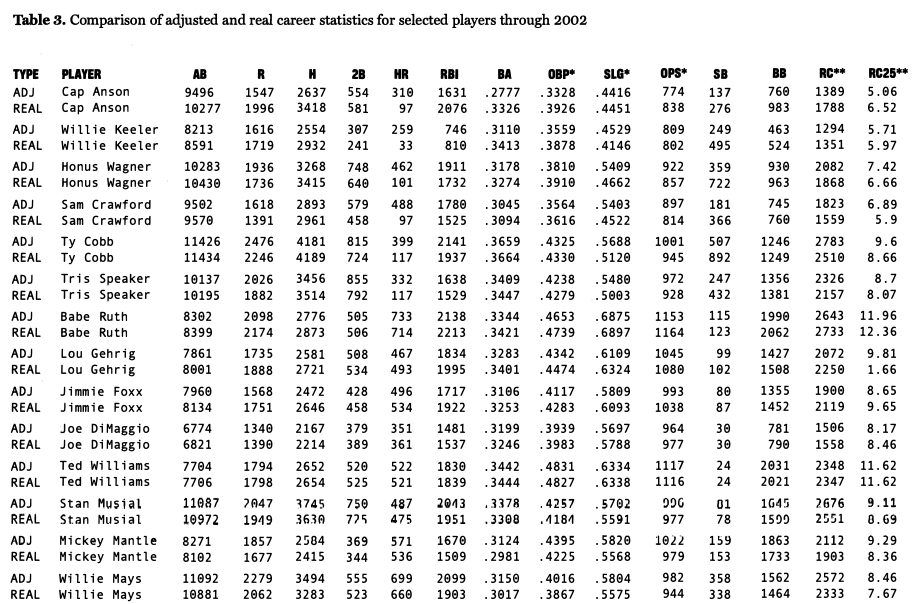
For post-1920 players, the most affected negatively overall seems to be Jimmie Foxx, who moves out of the 500 home run club (Real: .325/534/1,922/1,038 OPS (note OPS calculation includes hit by pitch, but not sacrifice flies) vs. Adjusted: .3ll/496/1,717/993 OPS). Foxx has the third largest decline in OPS (-45) among players with at least 1,000 career ABs — the first two being Todd Helton (-53) and Earl Averill (-52).

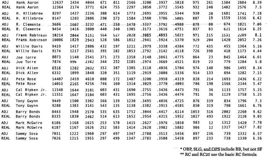
The most affected positively overall seems to be Dick Allen (Real: .292/351/1,119 914 OPS vs. Adjusted: .311/387/1,305 974 OPS). The players closest to their original stats are probably Ted Williams (Real: .344/521/1,839 1116 OPS vs. Adjusted: .344/522/1,830 1117 OPS), Cal Ripken (Real: .276/431/1,695 791 OPS vs. Adjusted: .276/431/1,690 791OPS), and Sammy Sosa (Real: .278/499/1,347 897 OPS vs. Adjusted: .279/497/1,347 897 OPS).

In terms of famous records, Hank Aaron’s HR record becomes 811. Three players join the 600 home run club (Frank Robinson (627), Harmon Killebrew (614), and Reggie Jackson (600)). Willie Mays just misses the 700 home run club with 699. Pete Rose gets 4,610 hits, 362 more than Ty Cobb (4,181). Hank Aaron comes much close to Cobb than in real life with 4,044 hits. Overall, 25 players now have at least 3,000 hits. This includes Frank (3,151) and Brooks Robinson (3,091); the only players to move into the 3,000-hit plateau who are not there in real life. Two players move out of the 3,000-hit plateau: Wade Boggs (2,982), who had 3,010 hits in real life, and Cap Anson (2,637), who had 3,418 hits in real life (a difference of almost 23%). Ty Cobb still leads in career average (still at .366). Tony Gwynn moves all the way up to fourth (.350), and Rod Carew moves to sixth (.341).

(Click image to enlarge)

 

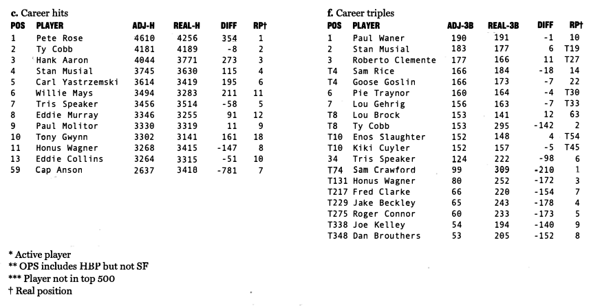
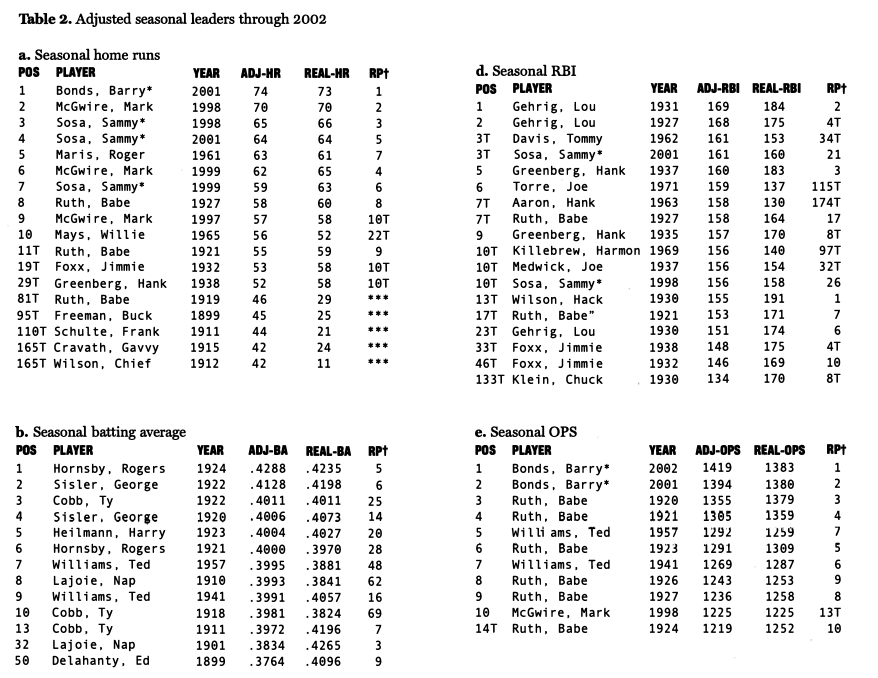
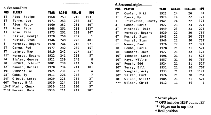
Table 1 shows the top 10 career leaders in various categories. Table 2 shows the leaders in various single-season categories (which are discussed below).

The top five pre-1920 players (defined for career leaders as those players starting their careers before 1910 or ending their careers before 1920), with their position in the overall leaders, are included in the career and single-season home runs list.

(Click image to enlarge)

 

In both of the tables, I’ve also included the rest of the real top 10 and their position on the adjusted list, if they did not appear on the adjusted list already. Triples are included in both tables because they are, without question, the most affected statistic (in terms of leaders) due to the Deadball Era algorithm.

For single-season records, no asterisk was necessary for Roger Maris, who now hits 63 home runs in 1961, five more than Babe Ruth’s 1927 total of 58. The clos­est to Ruth before Maris is now Ralph Kiner, who still hits 54 in 1949. Of the other players who came closest to Ruth in real life, Jimmie Foxx’s total of 58 in 1932 becomes 53, Hank Greenberg’s 58 in 1938 becomes 52, and Hack Wilson’s 56 in 1930 becomes 49. Mark McGwire still hits 70 in 1998, but the current record is now 74 by Barry Bonds instead of 73.

For RBI, Hack Wilson’s former total of 191 in 1930 is now no better than a tie for 13th with George Foster in 1977 (155). Lou Gehrig has the top two spots in RBI (169 and 168 in 1931 and 1927, respectively). Sammy Sosa is now tied for third place with Tommy Davis (161 in 2001 and 1962, respectively). Based on the Deadball Era algorithm, five players hit 40 home runs or more prior to 1920 (Babe Ruth (46 in 1919), Buck Freeman (45 in 1899), Frank Schulte (44 in 1911), Chief Wilson (42 in 1912), and Gavvy Cravath (42 in 1915).

Only four players hit .400 in a season (rounded to the nearest thousandth) a total of six times. Rogers Hornsby leads with .428 in 1924, 15 points ahead of George Sisler’s .413 in 1922. Hornsby and Sisler do it twice; Hornsby hits exactly .400 in 1921 and Sisler, in 1920, hits .401. The other players to hit .400 are Harry Heilmann (.401 in 1923), Ty Cobb (.401 in 1922 — while Cobb only hits .400 once, he hits over .390 no less than eight times), and Ted Williams (.3995) in 1957 (would Williams have considered that hitting .400?).

Williams also hit over .399 in 1941 (.3991 — Williams probably wouldn’t have been happy about that, either). In recent years, Tony Gwynn’s 1994 average becomes .397, George Brett’s average in 1980 becomes .393, and Rod Carew’s average in 1977 becomes .391. Also, Joe Torre hits .385 in 1971 and Barry Bond’s 2002 average becomes .382.

See Table 3 for a comparison of real and adjusted statistics for selected players.

FRANK CHIMKIN is Data Manager/Analyst for the Division of General Pediatrics, Columbia University. He has been a SABR member since 1993. He dedicates this article to his better half, Michele; his father, Stuart; and his late maternal grandfather, Irving Weisman.

 

(Click image to enlarge)

 

Notes

1. In the 2003-04 McFarland Baseball Books catalog alone, more than one dozen books are available which compare players and/or teams from one era to another.

2. Thorn, John, et. al., Total Baseball, 6th Edition, Total Sports, 1999, p. 2,534.

3. James, Bill, “Runs Created,” in Bill James, et. al., Bill James Presents Stats All-Time Major League Handbook, Stats, Inc., 1998, p. 7.

4. Note that, in this paper, the basic RC formula ((H+BB)x(TB) + (AB+BB)) is used for all years, regardless of the availability of data to com­plete the more advanced runs-created formulas.

5. For example, without going into the numbers, for many years of Babe Ruth’s career if you try to adjust his home runs to league averages and then compute them for a typical home run year in baseball history, Ruth comes out with more home runs than at-bats.

6. The algorithm is:

1. Games played remain the same
2. Batting outs (AB – H) remain the same.
3. The relationship between productivity as a hitter and the league average remains exactly the same.

To complete (3) find the difference between the team’s runs scored vs. 750. Multiply this index by the player’s real runs created to get the adjusted runs created. Then adjust this for park factor (which is modified based on the fact that half of the games are not played in that park). From there you enter the adjusted runs created in the hits formula (see methodology) to find the adjusted hits. Counting statistics rise and fall with hits. Productivity statistics (e.g., RBI, runs scored) rise and fall with runs created.

7. The Deadball Era algorithm includes the three elements of the first algorithm plus:

4. 67% of triples become home runs.

5. 3% of batting outs become home runs.

6. 2% of batting outs become doubles.

7. 50% of stolen bases disappear.

8. Hits are pegged at whatever level creates the appropriate level of offense (the change in runs created).

9. Everything else rises and falls with hits or total bases (as in the first algorithm).

10. Note that in order for the hits to come out right, you also must assume that 5% of batting outs are taken away from singles (in order for the batting outs to remain the same, those 5% of batting outs which have been allotted to doubles and triples must come from somewhere). James does not mention this in the text, however, so it is possible that he might have figured out some other way to account for the change in batting outs.

8. James arbitrarily chose 750 runs as what seemed to him to be a “normal context” for runs scored. However, according to my calculations since 1920 the average number of runs scored per team in both leagues is very close to 700 (699.6). I used 750 anyway to remain consistent with James. Note that for players who switched teams during the year, the runs scored for the entire year are used even though a larger or smaller proportion of the runs may have been scored during the time the player was with the team. Also, the 750 runs are based upon 162 games; so in games-shortened seasons (such as for strike, war, or pre-expansion years), players will not have their statistics altered as if a 162-game schedule was played.

9. When I attempted to check some of my results against those of James’s, the adjusted runs created were slightly off (59 for my analysis; 63 for James), thereby causing differences in the corre­sponding statistics. You can see these differences by checking the Adjusted Career Stats for Davis in Table 3 versus those in the James book on page 743. I believe this was due to the way James calculates park factors vs. the way the Lahman database does (I know that the Lahman database uses three-year park factors). When I plugged in the BPF for 1965 that James used for Davis (76 vs. 93 for the Lahman database) the adjusted runs created came out the same. Since 1965 was the only season that James mentions the BPF he used, it was the only season I could check.