Do Hitters Boost Their Performance During Their Contract Years?

This article was selected for inclusion in SABR 50 at 50: The Society for American Baseball Research’s Fifty Most Essential Contributions to the Game.

---

Each season, baseball fans and journalists alike identify which players are in the final years of their contracts because a lot rides on how the players produce in their “contract year.” Will a player boost his effort and performance in an effort to improve his value and bargaining power? Or will he crumble under the pressure? Or are players’ performances uncorrelated with where they stand in their contract cycles? Legendary manager Sparky Anderson believed players rose to the occasion in their contract years declaring, “Just give me 25 guys on the last year of their contract; I’ll win a pennant every year.”1 Although anecdotal evidence abounds, this paper uses a robust data set and appropriate player-specific econometric modeling highlighted in O’Neill to show that Anderson was right—players’ performances improve during their contract years.2 To find the answer requires following players throughout their careers to tease out changes predicated on contract status, rather than comparing players to one another given their contract status.

For example, in the last year of a three-year contract with the Mariners in 2006, Raul Ibañez sported an .869 OPS (on-base plus slugging percentage), up from .792 OPS the previous year.3 He subsequently signed an $11 million, two-year contract with the Mariners. In his next contract year, 2008, his OPS of .837 slightly exceeded his 2007 OPS of .831. Ibañez then signed a $31.5 million, three-year contract with the Phillies. At the end of that deal, in 2011, Ibañez’s .707 OPS dipped lower than his previous year’s OPS of .793 and the Yankees signed him to a one-year deal at $1.1 million. Two of Ibañez’s three contract years show boosts in performance, while the third demonstrates a significant drop. He was also 39 years old in 2011, suggesting age must be accounted for while searching for the answer.

The parties in contract negotiations—players, agents, and team owners—understand that incentives affect performance and that performance impacts pay and contract length. Players seek job security, income, and championships, while profit-seeking owners want players to perform well to win games and championships and secure fan enthusiasm. In contract negotiations, how a player has performed over his career serves as an imperfect predictor of his future performance. If players believe that team owners weigh a player’s most recent season more heavily than preceding years, it sets the stage for the contract year phenomenon. The attraction of a lucrative future contract provides ample incentive for a player to put in additional time and effort to boost performance in his contract year. After signing a new guaranteed contract, both pay and contract length are set regardless of actual performance, which removes the previous incentive.4 For longer-term contracts, this may lead to shirking. Eventually, a new contract year arrives and the incentive to boost performance reappears.

Difficulty arises in separating the individual performance of a baseball player from his team’s capabilities. This proves especially true for pitchers since decisions made about their pitch selection, pitch location, and strategy may depend on their team’s fielding proficiency and the strength of the bullpen. For a hitter, the type of pitch he sees may depend in part on the hitters adjacent to him in the lineup and the situation. This paper analyzes individual data on hitters (position players), rather than pitchers, while cognizant of the potential measurement errors. Adjusted OPS (OPS100) serves as the measure of the hitter’s performance. Although random variations in OPS100 from one year to the next can occur, it is unlikely for a large group of players that above average performances would randomly occur during contract years. I contend that effort and performance change from one year to the next depending upon where the player sits in his contract cycle.

Major League Baseball’s use of salary arbitration, contract extensions, and free agency provides avenues for enhanced contract conditions for players. This paper focuses on free agents with six or more years of MLB service for the following four reasons:

(1) free agency is associated with the greatest financial gains for players as teams bid for players’ services;

(2) at least six years of service enable more observations per player to capture more robust results;

(3) free agents with fewer than six years are those who have been demoted to the minors or released; and

(4) there will be a sufficient number of players who may retire at the end of their contract year, an intention that is expected to impact contract year performance.

Previous Research Findings

Previous research on MLB contract year performance shows mixed results. As detailed in O’Neill, the choice of performance measure and statistical technique employed often create contradictory results.5 Researchers generally analyze hitters, believing hitting statistics are less contaminated by team play than pitching statistics. The use of slugging percentage (SLG), at-bats (ABs), days on the disabled list (DL), wins above replacement player, OPS, and runs created per 27 outs (R27), show the range of offensive performance measures investigated. Given differences in players’ abilities, changes in a player’s output should be relative to his ability, indicating why several studies use the deviation between current and three-year moving average of a player’s offensive statistics to capture changes in a player’s output. A deviation-based model by Maxcy et al. finds no significant change in SLG for players in their contract year.6 Maxcy et al. does find that players seeking new contracts spend fewer days on the DL and have more ABs, contending they do so to make themselves more attractive to team owners. Birnbaum does not find a boost in R27 during contract years, whereas Perry does using WARP.7,8

Using ordinary least squares (OLS) regression enables one to predict changes in output during the contract year while controlling for observable player traits, such as age, years of MLB experience, team success, etc. However, compiling data on many players (cross sectional data) over several years played (time series data) creates a “panel” dataset. OLS estimation leads to biased results with panel data. Previous studies show robust statistical evidence of the contract year boost when using appropriate panel data estimation techniques, whereas those applying OLS models do not, as discussed in O’Neill.9 Analyzing data on hitters between 2001 and 2004, Dinerstein uses seemingly unrelated regression (SUR) and finds statistically significant increases in a hitter’s SLG during his contract year.10 Interestingly, from the team owners’ perspectives, Dinerstein finds that consistency of a player’s performance mattered more than the most recent performance. If teams are seeking consistency, they will pay for it, and players will begin to aim for steady hitting performances. If Dinerstein is correct, we should see a reduction toward zero in the magnitude of the contract year boost. Hummel and O’Neill employ fixed effects estimation with data on free agents playing 2004–08 and find 4.2–5.5 percent boosts in OPS during contract years.11 They note that players intending to retire no longer have financial incentive to boost effort, although they may desire to go out on top. Their results suggest the former effect dominates, shown by an 11.2 – 13.2 percent decrease in OPS for retiring players in the last year of their contracts, after controlling the diminishment of performance due to age and age-related injury.

Ability, Effort, and Performance

Team owners and general managers observe differences in players’ performances through easily available statistics. The difference between innate ability and effort, however, which together account for the differences in players’ performances, proves difficult to discern. In a given year, a player’s ability generally remains relatively constant, but his effort can change and lead to differences in performance levels. While unlikely that effort changes much during a game, offseason effort and effort between games in-season can vary. Players can exert effort to enhance their productivity by engaging in more intense workouts, restricted leisure activities, and eating healthier diets.

Players alter their effort when their interest dictates. If players believe team owners place greater weights on more recent performances, this motivates players to increase their effort and (ideally) performance during their contract year. But if players perceive that owners value consistent performance, then boosting performance in the contract year remains unlikely. When a player intends to retire at the end of the contract cycle, the incentive to perform and acquire another contract disappears, which is expected to reduce effort and performance during all years of the final contract, including the last year.

Multiple Regression Model to Estimate Adjusted On Base Plus Slugging Percentage

The dependent variable for this study is OPS100, preferred over OPS because it accounts for league play and the player’s home baseball park. This offensive measure accounts for power and reaching base frequently, two events contributing to scoring runs. OPS100 does not depend upon playing time and captures offensive prowess better than RBIs, batting average, HRs, etc.12 Albert and Bennett find OPS a better predictor of scoring runs than its two components separately.13 Barry Bonds holds the single-season record for unadjusted OPS at 1.4217 in 2004 when his SLG was .812 and his OBA was .609.14 During that season he typically walked or hit a home run during a plate appearance.

The suggested regression model for OPS100 for player i in season t is

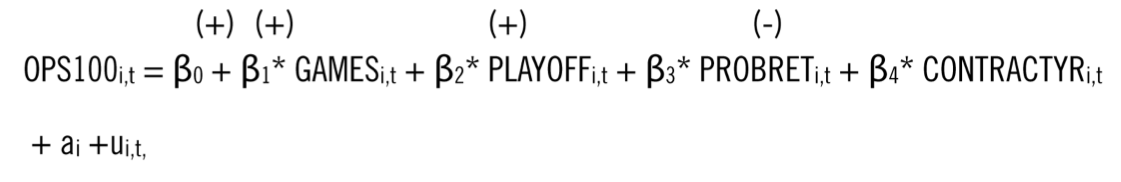
where: GAMES represents the number of games played; PLAYOFF is a binary variable equal to 1 when the player’s team makes the playoffs and 0 otherwise; PROBRET is the estimated probability of retirement; and CONTRACTYR is a dummy variable denoting whether season t is a contract year (=1) or not (=0). The sign above each β coefficient denotes the expected impact on OPS100 given an increase in the independent variable, holding all else constant. The stochastic error comprises two terms impacting a player’s performance: a_i is the unobserved player effect representing all time-invariant factors that cannot be measured or observed, such as innate ability, work ethic, drive, etc.; and µ_i,t represents random errors, due to accidents, weather, etc.15

The GAMES and PLAYOFF variables serve as control variables to mitigate potential bias. Playing more games helps a player gain confidence at the plate, likely raising his OPS100. Similarly, players with higher OPS100 statistics likely play in more games. The expected positive association between OPS100 and GAMES implies β₁ > 0. Several reasons suggest β₂ > 0. If a player’s team is in the playoff hunt, he is expected to boost his performance to help his team make the playoffs and potentially win a championship. Teams in a playoff race may trade for high performing hitters at the trade deadline, suggesting another reason for the positive association. A financial incentive to perform better also exists, since team members earn playoff revenues. Lastly, higher OPS100 figures may lead to teams making the playoffs.16

At the end of a player’s contract, he may or may not sign a new contract. He may willingly choose to retire, retire reluctantly due to advanced age or injuries, or be forced to retire because no team is willing to hire him despite his desire to keep playing. Unfortunately, it is not feasible to know which case prevails for all players. The variable NOPLAY=1 denotes a player is not on a MLB team the year after a contract year and NOPLAY=0 indicates he is on a roster. If NOPLAY switches from 0 to 1 because a player willingly chooses to retire, the expected impact is a decrease in OPS100 due to the lack of incentive to sign another contract. If NOPLAY switches for one of the other reasons for retirement, it may be due to a low OPS100, in which case the impact of NOPLAY on OPS100 is biased. To mitigate the bias and introduce the potential reasons behind retirement – advanced age, injuries, and poor performance, – a new variable that predicts the likelihood of retirement is created, PROBRET, following work by Krautmann and Solow.17 The estimated probability of retirement, discussed and shown later, is used to predict the retirement intention for each player for each year. Using PROBRET instead of NOPLAY as an independent variable reduces bias. Players who choose to retire do not seek another contract, therefore are expected to have a lower OPS100. Additionally, a player with a low OPS100 is more likely to have a higher probability of retirement as he goes unsigned or reluctantly hangs up his cleats. These suggest β₃ < 0.

MLB hitters are expected to engage in opportunistic behavior and increase their performance during the contract year, thus β₄ > 0. This presumes team owners value the most recent performance as a solid indicator of future performance, making way for the contract year boost. CONTRACTYR is the only independent variable in (1) that satisfies causal inference, rather than simply correlation, since a player’s contract status is known a priori.

Data

Data are collected on all free agent hitters playing during the most recently completed 2006-2011 Collective Bargaining Agreement (CBA) who had six or more years of MLB experience, a minimum of two years of observation, and played in at least seven games in a year. Choosing players under the same CBA helps reduce potential impacts due to changes in CBAs, since all players and team owners are subject to the same contract and free agency guidelines, and revenue-sharing rules.18 Signing new local and national TV contracts also affect revenue-sharing streams and hence salaries, but these are not captured in the data set.

Hitters with one-year and longer-term contracts are used. Players with longer term contracts generally represent those with higher ability; eliminating those with one-year contracts would potentially bias the results.19 Ultimately, 256 MLB free agent hitters meet the data selection criteria. The panel dataset is unbalanced, meaning the number of observations per player need not be the same.

ESPN.com’s Major League Baseball Free Agent Tracker lists the positions played, age, current team and new team unless re-signed, for all free agents in each year. Players who do not receive another contract are listed as retired or free agent again. Baseball-Reference.com provides OPS100 statistics, the number of games played each season, and the year in which a player debuted in the major leagues. Josh Hermsmeyer unselfishly provided me with the number of days on the disabled list (DL) for all players in 2006-2009 from his MLB Injury Report. Backseat Fan (2010) and FanGraphs (2011) provide the days on the disabled list for players in 2010 and 2011, respectively. For players who change teams via an in-season trade, the playoff status of the final team is used.

Table 1 presents the format of the unbalanced data set for two players. The first player is outfielder (POSITION=9) Bobby Abreu, given an identification code of 2, who was 32 years old in 2006. Abreu appears on MLB rosters in all six years of the 2006-2011 CBA and with the Dodgers in 2012, thus NOPLAY = 0 for all of his years. In his 2008 contract year and prior year, he played with the Yankees, having been traded from the Phillies in 2006. The Yankees made the playoffs in 2006 and 2007 but not in 2008, shown by PLAYOFF=1 and 0, respectively. In 2007, Abreu shows an OPS100 of 113 playing in 158 games, compared to his OPS100 of 120 in 156 games in his 2008 contract year. Abreu debuted in the majors in 1996, implying 11 years of experience (EXP) by 2006. With no days on the DL over the six years, DL=0.

 

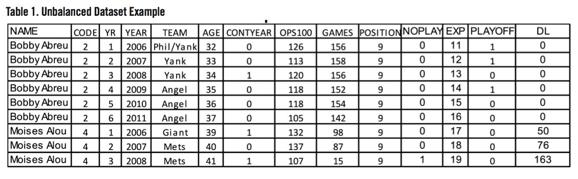
Table 1. Unbalanced Dataset Example
(click image to enlarge)

 

The second player, outfielder Moises Alou, shows two contract years, in 2006 with the San Francisco Giants and in 2008 with the New York Mets. He had 15 years of MLB experience by 2006 at age 39. Alou did not play on a MLB team in 2009, thus NOPLAY = 1 for 2008. His teams did not make the playoffs in any of the three years. Injuries led to increasing numbers of days on the DL and fewer games played between 2006 and 2007, and by 2008 two major injuries limit Alou’s playing time to only 15 games with 163 days on the DL. Three observations for Alou and six for Abreu indicate an unbalanced dataset.

Sorting the descriptive statistics by contract year status, interesting results appear in Table 2. The differences in means for all variables, except playoffs and days on the DL, are statistically significantly different at p<.001. There are 546 player-year observations for contract years and 470 for non-contract years. The average OPS100 for the contract year is 85.9 compared to 97.2 for the non-contract year, which appears contrary to the contract year boost hypothesis. This contrary result arises chiefly from the ex-post retirements (NOPLAY=1) of 23.1 percent in the contract year observations swamping the 3.2 percent in the non-contract year that may be due to poorer hitters receiving only one-year contracts. Ten fewer average games played in the contract year observations also suggests that less capable hitters have shorter contracts. Comparing the two means proves misleading and too simplistic. Predicting OPS100 via appropriate regression analysis can account for the influence of retirement and other factors to offer a more robust test of the contract year phenomenon.

 

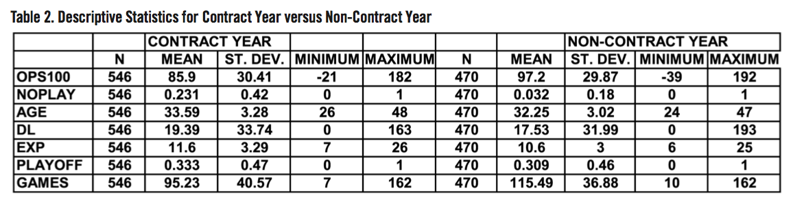
Table 2. Descriptive Statistics for Contract Year versus Non-Contract Year
(click image to enlarge)

 

Ordinary Least Squares versus Fixed Effects Estimation

Given panel data, estimation of the model via ordinary least squares (OLS) may be inappropriate due to omitted variable bias that occurs when immeasurable player characteristics in the error term a_i are correlated with some independent variables. For example, a player’s ability, captured in a_i, is expected to be positively correlated with the number of games he plays, GAMES, since higher ability players are likely to play in more games. Suppose higher ability players do have higher OPS100s and that playing in more games does increase OPS100. Ignoring the influence of ability, as in the case of OLS, means that GAMES receives more credit than warranted as the cause of the high OPS100. Consequently, the estimated coefficient of β₁ will be positively biased. Similarly, if a player has an exceptional (albeit non-measurable) work ethic, he will likely contribute more to his team success and increase his team’s chances of making the playoffs. This implies an expected positive correlation between a_i and PLAYOFF. If high OPS100s are attributable to both strong work ethics and playing on a playoff team, then the estimated coefficient of β₂ will also be positively biased in OLS.20 Eliminating bias requires a different technique, namely fixed effects (FE) estimation.

Studying a player’s motivation to perform across the contract cycle suggests concentrating on the within-player behavior. Estimating how each player alters his effort and performance over his contract cycle must be measured against his metrics, not against those of others. FE estimation calculates the mean of each variable over time for each player and subtracts it from the actual observation for each year to demean the data. For example, Bobby Abreu’s average OPS100 over his six years of playing is 116.5, which is subtracted from his actual OPS100 for each of his six years to yield six deviations or demeaned observations for his OPS100. After doing so for all players, the demeaned dependent variable of OPS100 is regressed on the demeaned independent variables via OLS producing the fixed effects within-player coefficients. Time-invariant unobserved traits in a_i, such as ability, have demeaned values of zero, eliminating them from affecting outcomes. Dropping out the unobserved traits via demeaning eliminates correlations and associated biases between unobserved traits and independent variables.21

While FE estimation addresses bias and focuses on changes in players’ behaviors, it comes with a cost. Finding statistical significance for estimated coefficients may be compromised. The variation in OPS100 across 256 players is expected to be much greater than the variation in OPS100 for individual players over their free agency careers. For example, the dataset shows a range in OPS100 from -39 to 192 with a standard deviation of 30.67, while Bobby Abreu’s only vary between 105 and 126 with a 7.09 standard deviation. Other players generally have smaller OPS100 deviations too. Since FE estimation concentrates on the within-player variation and dismisses the between-player differences in OPS100, it reduces the sample variation in OPS100 and lessens the likelihood of statistical significance for the estimated β coefficients. Demeaning the data also reduces the degrees of freedom by 255, further diminishing chances of statistical significance. Therefore, finding a statistically significant FE result for β₄, in spite of these perils, occurs because evidence from the dataset is compelling.

Estimating the Probability of Retiring

Players generally retire at the end of a contract. However, the predicted probability of retiring can change over time until actual retirement occurs and it should be considered by the team owner during negotiations. A player’s likelihood of retiring depends on how many years he has played, how many days have been spent on the DL, and his offensive performance per Krautmann and Solow.22 Equation (2) denotes the regression equation for the probability of retirement for player i in season t as

Players with more years of experience are expected to have increasingly greater likelihoods of retiring since they have signed several contracts and amassed income. Additionally, the aging process that accompanies years of experience takes its toll on bodies often coinciding with familial demands to be home more often. With EXP2 representing years of experience squared, α₁ > 0 and α₂ >0 are expected. More days on the DL are expected to increase PROBRET, i.e., α₃ > 0, since injuries inhibit playing ability and reduce interest by team owners. If a decline in OPS100 portends reduced future performance, it increases retirement likelihood, α₄ < 0. The stochastic error comprises both the unobserved time-invariant player traits a_i and unmeasured time-variant traits v_t such as family issues.

Using NOPLAY as the dependent variable, estimating (2) via FE leads to the linear probability model (3) below. Since NOPLAY is determined after the season, all of the independent variables yield causal inference. The p-values for one-tailed hypotheses tests for the estimated slope coefficients are in parentheses below the estimates.

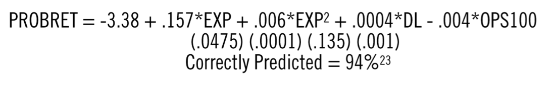
Days on the disabled list do not statistically predict likelihood of retiring, but remaining variables do. Each additional year of MLB experience increases the likelihood of retiring exponentially and a one point increase in OPS100 reduces it the probability of retirement by .4 percent. Since the -3.38 intercept pertains to the last player’s last year, the predicted output for all players for all years occur as changes from -3.38. For brevity, they are not provided.

For example, Bobby Abreu could have retired after his 2008 contract year, but his predicted probability was .001 (near zero) and he did not retire.23 His likelihood rose to 1.5 percent in 2009 due to his two-point decrease in OPS100 and extra year of experience. By 2010, despite no change in his OPS100 from 2009, the additional year playing leads to a probability of 12.7 percent. In 2011, his sixteenth year in the majors and drop in OPS100 to 104 increases his likelihood to 33 percent. For Moises Alou the model predicted a 60 percent chance of retirement following his 2008 season, when he did in fact retire. The predicted values of PROBRET for all 1,106 observations are calculated and ultimately used to estimate (1).

Results from Estimating OPS100

Regression model (1) derives from two improvements in the model estimated in O’Neill.24 First, traditional theory suggests that as players age, their offensive performance increases at a decreasing rate as they become more comfortable in hitting, until it peaks, and eventually declines as age depreciates hitting skills. O’Neill includes the quadratic form of age, AGE and AGE squared, as independent variables impacting OPS100.

Additionally, O’Neill’s PROBRET estimation employs performance, injury, and the quadratic form of years of experience in place of age. O’Neill finds the odd result that OPS100 increases at an increasing rate after age 33. Having age enter PROBRET through its correlation with years of experience, and then using PROBRET along with age in predicting OPS100, may have led to that usual result. Second, O’Neill segregated catchers and shortstops as defensive players, believing that they sport lower OPS100 statistics in exchange for better defensive play. However, since FE estimation demeans the data and players who are shortstops or catchers generally do not change positions, it does not seem appropriate to segregate them.

The 1,016 player-year observations yielding equation (4) presents the FE multiple regression equation for predicted OPS100 (OPS100^) with one-tailed p-values in parenthesis.25 The Buse-R2 indicates that 78 percent of the variation in adjusted OPS is explained by the model with these independent variables.26 Games played and being on a playoff team indicate the expected positive sign, but they are not statistically significant at 5 percent.

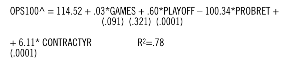
The highly significant PROBRET coefficient says that a one percentage point increase in the likelihood of retiring reduces expected adjusted OPS by 1.0034 points or 1.1 percent decline relative to the mean OPS100 of 91.12. A 10-percentage point increase in the likelihood of retiring, about one half standard deviation in PROBRET, reduces predicted adjusted OPS by 10.034 points.

The estimated model provides evidence of the contract year phenomenon, but the phenomenon depends upon the likelihood of retirement. If a player is in a contract year, holding all else constant, the expected increase in his adjusted OPS is 6.11 points or 6.7 percent increase relative to the mean. But for two otherwise identical players, one in his contract year and the other not, the expected OPS100 for the former is 6.11 points higher. Using the Grossman heuristic that every .100 increase in OPS raises salary by $2,000,000 and converting OPS to OPS100 enables monetizing the 6.11 bump. 27 The contract year boost is expected to increase annual salary by $470,000, about 15.2 percent of the average salary of $3.1 million in 2011.

The impact from the likelihood of retiring offsets the contract year boost. Each additional percentage point increase in a contract year player’s retirement probability reduces the 6.11 boost by 1.0034. A complete offset of no expected change in OPS100 during the contract year occurs with a jump in retirement likelihood of about 6.1 (6.11/1.0034) points. With years of experience driving retirement likelihood exponentially, a decline in expected OPS100 reasonably appears at the end of contracts for players with many years of experience. For instance, a 10-point increase in the probability of retirement leads to a 3.9 (6.11-10.034) decline in expected OPS100 during a contract year.

Conclusions

By using FE estimation to account for changes in each player’s behavior and reducing bias due to unobserved player traits pervasive with OLS estimation, the data show strong support for the contract year boost. From FE estimation, two important contract year findings follow. First, the adjusted OPS of a free agent hitter in his contract year is expected to be 6.7 percent greater than in non-contract year periods—higher than previously noted studies. Second, “retiring” players show a decline in their contract year performance and any models which ignore retirement will be misspecified. OLS estimation of the same dataset (not shown) yields a negative impact on OPS100 during the contract year, albeit not statistically significant. This biased result coincides with the contrary findings in Table 2 that show lower average OPS100 for contract year observations than non-contract year observations.

The model may prove helpful during contract negotiations as one can compare a hitter’s actual performance relative to expectations. Take Albert Pujols as an example. In 2008 and 2009, his OPS100 statistics of 192 and 189 greatly exceeded his predicted statistics of 175 and 176, respectively. In 2010, his OPS100 dropped to 173 to his expected value. In 2011—his contract year—the model predicts an OPS100 of 155, yet he hit only 148. Despite two years of declining OPS100 values that failed to meet the model’s expectations, the Angels still signed Pujols to a 10-year, $240 million contract. His OPS100 has continued to decline, dropping to 138 in 2012 and 117 in 2013. This type of post-contract performance leads me to the next related research project: whether players shirk after getting a new long-term contract.

HEATHER M. O’NEILL is a Professor of Economics at Ursinus College in Collegeville, Pennsylvania. Entering her 28th year at Ursinus, all of her students know she is an active athlete and a survivor of the 1964 Phillies collapse. While still an avid Phillies fan with a place in her heart for Johnny Callison, she serves as the “Cookie Rojas” in her department by teaching a variety of applied microeconomics courses, including the Economics of Sports. Joining SABR in 2011 opened her eyes to the trove of available data that will engage and excite her for years to come.

 

Notes

1 John Lowe & John Erardi, “Baseball Hall of Fame Manager Sparky Anderson Dies at 76,” USA Today, http://usatoday30.usatoday.com/sports/baseball/2010-11-04-sparky-anderson-obit_N.htm (accessed July 20, 2014.)

2 Heather O’Neill, “Do Major League Baseball Hitters Engage in Opportunistic Behavior?” International Advances in Economic Research, 19(3), (2013), 215-232.

3 Baseball-Reference.com. “Major League Baseball Statistics and History,” Sports Reference LLC. http://www.baseball-reference.com/players (accessed September 28, 2012).

4 Players with year options or incentive clauses written into contracts maintain motivation to boost performance.

5 Heather O’Neill, “Do Major League Baseball Hitters Engage in Opportunistic Behavior?”

6 Joel Maxcy, Rodney Fort, and Anthony Krautmann, “The effectiveness of incentive mechanisms in Major League Baseball,” Journal of Sports Economics, 3(3), (2002), 246-55.

7 Phil Birnbaum, “Do Players Outperform in Their Free-agent Year?” http://philbirnbaum.com (accessed April 27, 2009).

8 Dayn Perry, “Do Players Perform Better in Contract Years?” Baseball Between the Numbers (New York: Basic Books, 2006), 199-206.

9 See Heather O’Neill, “Do Major League Baseball Hitters Engage in Opportunistic Behavior?” for differences in outcomes due to OLS versus FE estimation.

10 Michael Dinerstein, “Free Agency and Contract Options: How Major League Baseball Teams Value Players,” PhD. Dissertation, Stanford University. May 11, 2007.

11 Matthew Hummel and Heather O’Neill, “Do Major League Baseball Hitters Come Up Big in Their Contract Year?” Virginia Economics Journal, 16, (2011), 13-25.

12 Jonah Keri, “What’s the Matter with RBI? .and Other Traditional Statistics,” Baseball Between the Numbers. (New York: Basic Books, 2006), 1-13.

13 Jim Albert and Jay Bennett, “Curve Ball: Baseball, Statistics, and the Role of Chance in the Game” (New York: Copernicus Books, 2001).

14 Baseball-Reference.com. “Major League Baseball Statistics and History” Sports Reference LLC. http://www.baseball-reference.com/players (accessed September 28, 2012).

15 One could include vt in the error term to denote time-variant, unobserved or measured traits such as changes in family structure. The effects were tested econometrically, found to be insignificant, and excluded in (1). Lawrence Kahn, “Free Agency, Long-Term Contracts and Compensation in Major League Baseball: Estimates from Panel Data,” The Review of Economics and Statistics, 75(1), (1993), 157-164.

16 Playoff teams generally have better players and their surrounding presence can enhance a hitter’s performance, which introduces the aforementioned measurement error associated with seeking an individual’s performance.

17 Anthony Krautmann & John Solow, “The Dynamics of Performance over the Duration of Major League Baseball Long-term Contracts,” Journal of Sports Economics, 10(1), (2009), 6-22.

18 Although the CBA was signed at the end of the 2006 season, I include player observations from 2006. As noted at the time, the negotiations taking place during the 2006 season proceeded without much acrimony, in fact yielding ratification prior to expiration of the previous CBA. I am assuming the players were aware and in agreement of what the new agreement would bring, thus working with shared expectations and incentives. See “MLB players, owners announce five year playing deal” http://sports.espn.go.com/mlb/news/story?id=2637615 October 25, 2006.

19 Lawrence Kahn, “Free Agency, Long-Term Contracts and Compensation in Major League Baseball: Estimates from Panel Data,” The Review of Economics and Statistics, 75(1), (1993), 157-164.

20 See Heather O’Neill, “Do Major League Baseball Hitters Engage in Opportunistic Behavior?” for in-depth analysis of bias mitigated by FE estimation.

21 Unfortunately, the impact of time-invariant observable traits, such as race, height, etc. cannot be estimated since they too would drop out of the demeaned variables.

22 Anthony Krautmann & John Solow, “The Dynamics of Performance over the Duration of Major League Baseball Long-term Contracts,” Journal of Sports Economics, 10(1), (2009), 6-22.

23 To preclude predicted linear probabilities below zero, all negative predictions are assigned a probability of .001, essentially zero.

24 Heather O’Neill, “Do Major League Baseball Hitters Engage in Opportunistic Behavior?”

25 The Hausman test with p<.0001 rejected random effects in favor of fixed effects. Random effects assumes no correlation between traits in a_i and any independent variables.

26 When ex-post retirement, NOPLAY, is used instead of the predicted probability of retirement, the Buse-R2 falls to .68, suggesting less predictive power.

27 Mitchell Grossman, Timothy Kimsey, Joshua Moreen & Matthew Owings, “Steroids in Major League Baseball” (2007), http://faculty.haas.berkeley.edu/rjmorgan/mba211/steroids%20and%20major%20league%20baseball.pdf (accessed October 23, 2012).