

Going Beyond the Baseball Adage ‘One Game at a Time’: A Geek’s Peek at Streaks
This article was written by Ed Denta
This article was published in Spring 2024 Baseball Research Journal
Professional baseball players and coaches shrug off questions from reporters about the future with responses such as “all our focus is on winning today’s game” or “we’ll worry about the next series when we get there.” The media and fans, however, are mesmerized by historical statistics and records, with particular attention paid to streak records on the verge of falling, such as “the Atlanta Braves have now homered in 26 consecutive games and are threatening the all-time mark of 31 set by the 2019 New York Yankees,” as reported by MLB network during the 2023 All-Star break. The Braves eventually got to 28 games but were held homerless by the Chicago White Sox in an 8–1 defeat on July 16.
As a lifelong baseball aficionado, my interest in baseball history, trivia, and statistics has grown with each passing season. After the Baltimore Orioles started the 1988 season with 21 consecutive losses, the 2002 Oakland A’s ran off 20 consecutive wins, and the 2017 Cleveland Indians coupled streaks of 22 and five games to win 27 of 28 late in the season, I became fascinated with baseball’s winning and losing streaks. How often and when do they occur? Do they follow patterns? Are they predictable?
My aspiration is to combine a) my passion for baseball statistics and numbers, b) my experience as an engineer using database programs and Excel, and c) my extreme attention to detail, to contribute something unique to the annals of baseball analysis.
This research paper represents an in-depth analysis of all winning and losing streaks in the American and National Leagues since 1901. A reader with only limited knowledge of probability theory should still be able to understand the concepts and appreciate the results of this never-before-seen analytical picture of streaks.
RESEARCH PROCEDURES
The research set begins in 1901 with the advent of the American League (AL) as a major league. In 1901, the American League and National League (NL) each had eight teams, with teams from both leagues in Boston, Chicago, and Philadelphia, and by 1903 in the New York metro area. As of 2024, MLB has 30 active franchises playing from coast to coast. Through 2023, 206,711 games have been played.
Obtaining and Formatting Game Results. Game results (win, loss, tie) for all games and all teams in sequence came from Baseball Reference and Retrosheet. I then developed and applied a proprietary conversion scheme using Excel, to replace each win, loss, and tie with an encoded numerical value. This new dataset facilitates all filtering and parsing necessary to extract and analyze winning and losing streaks.1
Identifying Analysis Objectives. After encoding all win-loss-tie data, I next had to decide what streak attributes to research and extract. The results had to be both innovative and appealing to baseball fans, and particularly a baseball audience primarily of SABR members. In the end, my analysis produced two papers. This paper explains the mathematical theory behind winning and losing streaks and develops predictive equations, then compares the prognostications to actual streak results. The second paper, not presented here, explores streak data from a historical perspective.
STREAKS DEFINED
Winning streaks consist of sequences of consecutive wins or ties. Losing streaks consist of sequences of consecutive losses or ties. For purposes of this paper, ties are considered a neutral result. Ties neither terminate a streak nor extend the length of the streak. As a result, the nine-game sequence WWWTWWTWW is considered a seven-game win streak. Likewise, LLTTLLL is a five-game losing streak.

Of the 206,711 games played, 777 resulted in a tie with no winner determined. Ties were quite common in the first half of the twentieth century, with 82.5% of the tie games occurring by 1950. The last tie game occurred on September 29, 2016, between the Chicago Cubs and the Pittsburgh Pirates, when play was halted due to rain in the top of the sixth inning with the score tied, 1–1. The game was called and not suspended since it was late in the season and the result would have had no effect on the National League standings. Table 1 depicts the number of tie games by decade.
Going forward, all references to the number of games or decisions played denote only non-tie results, i.e. wins or losses. Games are played. Decisions are the team results of the game. Each team gets one result per game played and each game played produces two decisions for the league. The number of games and the number of decisions is the same (and interchangeable) when referring to a single team.
Preference for Seasonal Streaks. Streaks are characterized as either seasonal or wraparound. Seasonal streaks are confined to a single season, while wraparound streaks extend from one season to the next if the final non-tie result (either W or L) of Season n matches the first non-tie result of Season n+1. Only seasonal streaks are considered in this paper.
Measure of Streakiness. Streakiness is defined as the state or condition of being streaky. Streaky can be described as having streaks. To evaluate the positive and negative streakiness of a team during a given season, consider these new metrics and definitions:
- Streak Wins (SW) is the number of wins during a season that are part of winning streaks of five or more games.
- Streak Losses (SL) is the number of losses during a season that are part of losing streaks of five or more games.
- Win Streak Quotient (WSQ) is defined as Streak Wins (SW) divided by total wins (TW).
- Loss Streak Quotient (LSQ) is defined as Streak Losses (SL) divided by total losses (TL).
- Total Streak Quotient (TSQ) is defined as Streak Wins (SW) plus Streak Losses (SL) divided by Total Decisions (D).

Example: A team with a 97–64–1 record, with win streaks of 6, 9, 5, 5, 13, and 12 and loss streaks of 5, 7, and 5 has a WSQ of .515, an LSQ of 0.266, and a TSQ of 0.416.

MATHEMATICAL THEORY
Derivation and Calculations of Expected Streaks (50–50 scenario).
To gain a mathematical understanding of how often winning and losing streaks occur, let’s review some elementary probability theory. The chance of tossing a single coin and getting a specific result (either heads or tails) is 1 out of 2, or 0.5. The chance of getting a specific sequential result when tossing two coins (either HH, HT, TH, or TT) is 0.5 times 0.5, or 1 out of 4, or 0.25. Three coins yields 1 out of 8, or 0.125, and so on. To generalize, tossing a coin K times yields 1 of 2K sequential results. The probability, PK, of getting any one specific result is ½ times ½…times ½ a total of K times, which is the value ½ raised to the power of K. Equation 4 shows this expression algebraically, where K is the number of independent coin tosses:
The probability of a baseball team getting all wins in K consecutive games against another team is equivalent to tossing a coin K times and getting all heads, assuming each team has a one in two chance of winning each game.
Every win streak has a defined beginning and end. For a five-game win streak at the beginning of the season the game sequence is WWWWWL, during the season it is LWWWWWL, and at the end of the season it is LWWWWW. Note that except for the beginning and end of the season, the required decision sequence has an L before and an L after the string of five W’s. This seven-game decision string is the test sequence (TS) for a five-game win streak. A six-game win streak requires an eight-game test sequence. To generalize, an S-game streak (either winning or losing) requires an S+2 length test sequence. Therefore, TS=S+2.
Let’s determine how many times a win streak of five games (S=5) can be expected in a game sequence of 162 games (N=162) for a single team. The appropriate test sequence to identify a five-game win streak is LWWWWWL. The length of this test sequence (TS) is 7. Figure 1 depicts a WL game sequence of 162 games. To detect all five-game win streaks, the seven-game test sequence must be slid sequentially left to right across all 162 games.
Test 1 aligns the first W of the test sequence (its second entry) with Game 1. Note that only four of the necessary six entries for this first test location are a match, shaded test sequence entries 2, 4, 5, and 6. The first entry for Test 1 is given a match, since there is no corresponding decision in the game sequence, therefore, a five-game win streak is not detected in the first five games by Test 1.
Test 2 slides the test sequence one game to the right. Again, four entries match: 3, 4, 5, and 6.
Test 3 slides the test sequence another game to the right. In this case all seven entries in the test sequence match the game sequence, thereby detecting the first five-game win streak. This slide right process continues until the five wins in the test sequence align with the final five games in the game sequence as indicated by Test 158. Note that Test 155 detected a second five-game win streak near the end of the game sequence (Game No. 154 through Game No. 160).
Since a streak can occur at either the beginning or the end of a game sequence, the number of required tests (T) for an N-game sequence is T=N-S+1, where S is the streak length. From Figure 1, 158 tests are required to detect all five-game win streaks in 162 decisions, T=162-5+1=158.
To generalize, for a .500 team the expected number of S-game win streaks, EWS, in a decision sequence length of N is calculated by multiplying the required number of tests, T, by the probability of the test sequence, TS, matching the game sequence.

For very large values of N compared to S, Equation 5 simplifies to

For the case shown in Figure 1, S=5, TS=7, and N=162, therefore EWS=(162-5+1)/(27)=158/128 =1.234. One way to interpret an EWS of 1.234, is to say that there are 5-to-4 odds that a .500 team will have a single five-game win streak in a 162-decision sequence. This special case corresponds to a decision sequence of a team with equal probability of winning and losing (50–50), Therefore, expected loss streaks ELS equals EWS, 1.234 for a five-game losing streak.

The expected number of total S-game streaks, ETS, is given by Equation 7 where ELS=EWS for a .500 team.
![]()
In the example above, the .500 team can be expected to have 1.234 five-game winning streaks and 1.234 five-game losing streaks for a total of just under 2.5 five-game streaks in the 162-game season. Obviously fractional (non-whole) numbers of streaks are not possible. This concept is established in the short run so it can be understood and applicable in long runs of thousands of games.

Table 2 evaluates Equation 7 and shows the expected combined number of total streaks, ETS, by streak length (S) for various sizes of game sequences for a team with a 50 – 50 chance to win each game.
Calculation of Expected Streaks (Non 50–50 scenarios). Equation 7 shows the Expected Number of total streaks (ETS) for a team having a 50–50 chance of winning each game. Expected win streaks (EWS) and loss streaks (ELS) each make up half the total (ETS). Let’s examine the changes when the team is better than a .500 club.
Let PW be the probability of a win and PL the probability of a loss. PW and PL are both greater than 0 and less than 1 and sum to 1. Let’s generalize Equation 6, EWS=N/(2TS). The value two in this equation is the number 1 divided by the probability of a win, PW, or 1/PW, which equals two for a .500 team.
![]()
PW is the probability of a win and (1/PW) is multiplied TS times (the required length of the test sequence) in the denominator.
An S-game winning streak must have a loss right before and a loss right after the win streak in the test sequence. EWS now becomes
![]()
where 1/PL appears twice in the denominator and 1/PW appears S times (the streak length).
The generalized expected number of S-game winning streaks in N games for a team with a PW win probability and PL loss probability is as follows:

The generalized expected number of S-game losing streaks in N games for a team with a PW win probability and a PL loss probability is as follows:

The generalized total expected number of S-game streaks in N games for a team with a PW win probability and a PL loss probability is as follows:

Table 3 evaluates Equations 8, 9, and 10 to show the expected number of streaks in 100,000 games by streak length S, for Teams A, B, and C with win probabilities (PW) equal to .400, .500. and .550, respectively.

Team B’s (PW=.500) total winning streaks are equal to its losing streaks, 1,562. Not surprisingly, Team A’s (PW=.400) total losing streaks exceed its winning streaks, 3,110 to 614. While Team C’s (PW=.550) total winning streaks exceed its losing streaks, 2,265 to 1,015. The more a team’s PW deviates from .500 the greater the number of expected total streaks, ETSG. Streak totals of 3125, 3280, 3725 for Team B, C, and A, with deviations of .000, .050. and .100 independent of direction. The greater the performance diversity from .500, the more total streaks.
Equation 8 expresses the expected number of win streaks for only one streak length, S, to occur in N games. To calculate the expected number of total win streaks, EWSGS in N games, Equation 8 must be summed for all streak lengths of interest. This research paper is focused on all streaks from five to 26. Expected streaks of greater than 26 games are minuscule for less than 500,000 games.
Therefore, the Expected Number of Total Win Streaks for all streak lengths S, EWSGS, is expressed as

Similarly, the Expected Number of Total Loss Streaks for all streak lengths S, ELSGS, is expressed as

The expected number of total streaks, both winning and losing for all streak lengths S, ETSGS, is:

The previous discussion applies to the evaluation of streaks for a single team. Since there are two decisions for each game played, the number of games, N, must be replaced by the number of decisions, D, when evaluating league-wide streaks. Therefore, when considering league-wide results, equations 8a, 9a, and 10a become equations 8b, 9b, and 10b respectively.

Equations 8b, 9b, and 10b are called the expected streak equations.
Through this point in the paper, we have developed a lot of equations. Figure 2 clarifies equation nomenclature.

A consolidated listing of all expected streak equations is shown below.

Simulations.There have been 411,868 non-tie decisions in the AL and NL from 1901 through 2023. The 206,711 games played, minus 777 ties, equals 205,934, times two decisions per game, equals 411,868 decisions.
To verify the derived Expected Streak calculations in Equations 8b and 9b, multiple game simulations were run (and averaged) using Microsoft Excel 365. Ten columns of 411,870 random numbers evenly distributed between zero and one were populated using the RAND() function to create 10 independent simulations of 411,870 decisions. The RAND() function uses the Mersenne Twister algorithm (MT19937) to generate random numbers. Decision thresholds were imposed on each cell to render a win or a loss. To simulate streaks for a team with a .550 win probability, all random numbers between 0 and .450 were deemed a loss and all random numbers from greater than .450 to 1.000 were deemed a win. The sequence of wins and losses were evaluated and counted for streaks of various lengths. Simulation results were compared to results obtained by evaluating Equations 8b and 9b for various win probabilities for 411,870 decisions. The logarithmic chart in Figure 3 displays the results for two different win probabilities, .500 (50_50 case) and .600 (60_40 case).
Note that the simulation and predictive curves are nearly exact through the 16-game streak for the 50_50 case and through 21 games for the 60_40 case. The deviation beyond these points is due to limited simulation data. Evaluating more decisions and/or running and averaging more simulations would drive the simulation to converge with the prediction at the longer streak lengths. Despite this slight deviation, the simulations confirm the validity and accuracy of the predictive analysis.

(Click image to enlarge)
STREAKINESS AND PERFORMANCE DIVERSITY
Streakiness. Previous analysis and simulations have demonstrated that higher win probabilities produce more total streaks (and increased streakiness). Let’s test this hypothesis against actual data by examining the 123 years of historical win-loss records in our dataset. Higher win probabilities are manifested in the real world by greater performance diversity among the competing teams.
Expanding upon Table 3, Figure 4 summarizes the results of Equations 8a, 9a, and 10a for the Expected Number of Summed Win Streaks, EWSGS, Expected Number of Summed Loss Streaks, ELSGS, and the Expected Number of Summed Total Streaks, ETSGS, in 100,000 games, N, for a team’s Winning Averages, PW, from .500 to .660.
Note that EWSGS=ELSGS=3,125 for PW=.500. As PW increases, EWSGS and ETSGS increase while ELSGS decreases. This is as expected: the better the team, the better the chances for additional win streaks and fewer loss streaks. For a good team, win streaks increase at a higher rate than loss streaks decrease, resulting in more total streaks. A team with a .600 winning average will have 99% more win streaks (3,110 to 1,562), 61% fewer loss streaks (614 to 1,562), and 19.2% more totals streaks (3,725 to 3,125) of five or more games in 100,000 decisions than a .500 team.
Based on this analysis and backed by simulations, expect more total streaks of five or more games (and more streakiness) in seasons when teams have greater talent and performance diversity than when there is more parity. Let’s determine if this has been the case for 1901–2023.
Total Streak Quotient (TSQ, see Equation 3) is used to assess the seasonal streakiness of past results. TSQ is a normalized metric that scales streak results by the number of decisions in the space being analyzed. This allows for direct comparison between teams and seasons, independent of the number of games played or teams in the league.
Streak Wins (SW) is the number of wins during a season that are part of winning streaks of five or more games. Streak Losses (SL) is the number of losses during a season that are part of losing streaks of five or more games. Each game played by a single team results in one decision for that team. Equation 3 still applies when evaluating TSQ for the entire league, since each game played results in two decisions, a win to one team and a loss to the other.
Figure 5 displays the seasonal Total Streak Quotient (TSQ) for all of baseball.

The seasons with the highest TSQ, 1906, 1908, 1927, 1930, 1939, and 1953, all exceed .275. The lowest TSQs, all below .175, occurred in 1934, 1959, 1983, and 2014.
Figure 5 shows a large spike in streakiness since 2014. This could be due in part to “tanking.” According to Forbes, “tanking refers to the practice of a team deliberately fielding a lesser line-up for an entire season in order to extract a better position in the next amateur draft.” It might also involve trading or selling off high-priced aging veterans to depress payroll and better position the organization for future spending. These management practices can result in miserably deficient teams becoming league leaders in just a handful of seasons, as with the Houston Astros. The Astros lost 324 games from 2011 to 2013, but starting in 2015 made the playoffs in eight of nine years, won more than 100 games four times, appeared in four World Series, and won two (2017 and 2022). The Chicago Cubs had a similar turnaround. They lost 377 games from 2011 to 2014, but beginning in 2015, made the playoffs five of six ensuing years and won the World Series in 2016.
The three biggest losers in 2021, the Baltimore Orioles (110 losses), Arizona Diamondbacks (110), and Texas Rangers (102) all had considerable success in 2023. The Orioles had the best record in the American League, winning 101 games, while the Diamondbacks and Rangers both made the playoffs as wild-card teams and then faced each other in the World Series. Although lower than 2022, TSQ for 2023 (0.214) was still well above the linear trendline.
Performance Diversity. AVGDEV is used to quantify performance diversity. AVGDEV, Average Deviation, is defined as the average of the absolute deviations (DEV) of the winning average for all teams in the league from the mean for a given season. Since all times in both leagues are considered, the mean is .500 (i.e., total wins for the season equals total losses). To determine the deviation for each team, its winning average (PW) is subtracted from .500 and the result taken as a positive number (i.e., greater than 0). The positive deviation for all teams is then averaged, to produce AVGDEV for the season. The greater the performance diversity, the greater the AVGDEV. Figure 6 depicts the seasonal AVGDEV.

The seasons with the greatest team performance diversity mostly occurred early in the twentieth century: 1904, 1906, 1909, and 1954. The seasons with the most parity have all occurred since the late 1950s: 1958 and 1984.
Since the big leagues expanded to 30 teams in 1998 (ignoring the COVID-19 shortened 2020 season), there have been 84 instances of a team either winning or losing 100 games. Here is the breakdown by nine-year increments: 1998–2006: 29 times, 2007–15: 14 times, and 2016–23 (only eight years): 41 times. This indicates significantly more performance diversity 2016–23 than 2007–15.
Streakiness Vs. Performance Diversity. Figure 7 merges analyses of streakiness, TSQ, and performance diversity, AVGDEV, from Figures 5 and 6 to graphically demonstrate the correlation.
Note the obvious correlation between the two plots. More performance diversity, higher AVGDEV, begets more streakiness, higher TSQ. Also note the similarity between the two five-season moving average trendlines. It is apparent that there is less performance diversity and less streakiness (i.e., lower TSQs) in baseball beginning in the mid-1950s continuing through 2014, with an uptick beginning in 2015.
Another way to visualize the correlation between performance diversity, AVGDEV, and streakiness, TSQ, is with a scatterplot (AVGDEV on horizontal axis and TSQ on vertical axis) as shown in Figure 8, where the upward dashed linear trendline clearly demonstrates that more performance diversity leads to more streakiness.

The two most significant outliers were 1914 and 1934 (highlighted by perpendicular lines to the trendline). 1914 had middle diversity (AVGDEV of .061 against a mean of .069) and high streakiness (TSQ of .268 in contrast to a mean .219). At the other extreme, 1934 had high diversity (AVGDEV of .080 against a mean of .069) and low streakiness (TSQ of .170 against a mean of .219). These results are somewhat noteworthy as outliers, but not totally unexpected due to the relatively small sample size of only about 2,450 decisions per season.
The 1909 season clearly stands out as the prime season that validates the hypothesis that greater performance diversity (manifested by higher winning averages) produces more total streaks (and increased streakiness). This season has both the highest all-time performance diversity (AVGDEV) and Total Streak Quotient (TSQ), .109 and .303, respectively. At the opposite end of the spectrum is 1959, with very low values for AVGDEV (.045 in 1959 against a minimum .039 in 1958) and TSQ (.172 in 1959 against a minimum .165 in 1983).
Table 4 lists the seasonal values of the performance diversity measure, AVGDEV, and the streakiness metric, TSQ, for both the pre- and post-expansion eras (data plotted in Figure 8).
The down and up arrow icons highlight the bottom and top 20 percentile (i.e., 25 seasons) for each measure. Note the correlation between AVGDEV and TSQ. There are 14 instances in the 123 seasons where both measures are in the top 20% and eight instances for both in the bottom 20%. Even more glaring is the discrepancy between pre- and post-expansion values. All 25 of the highest performance diversity seasons and 23 of the 25 highest streakiness seasons (only exceptions being the early expansion years of 1961 and 1962) occurred prior to 1956. All 25 of the lowest performance diversity seasons and 22 of the 25 lowest streakiness seasons (exceptions 1923, 1934, and 1947) occurred after 1957.
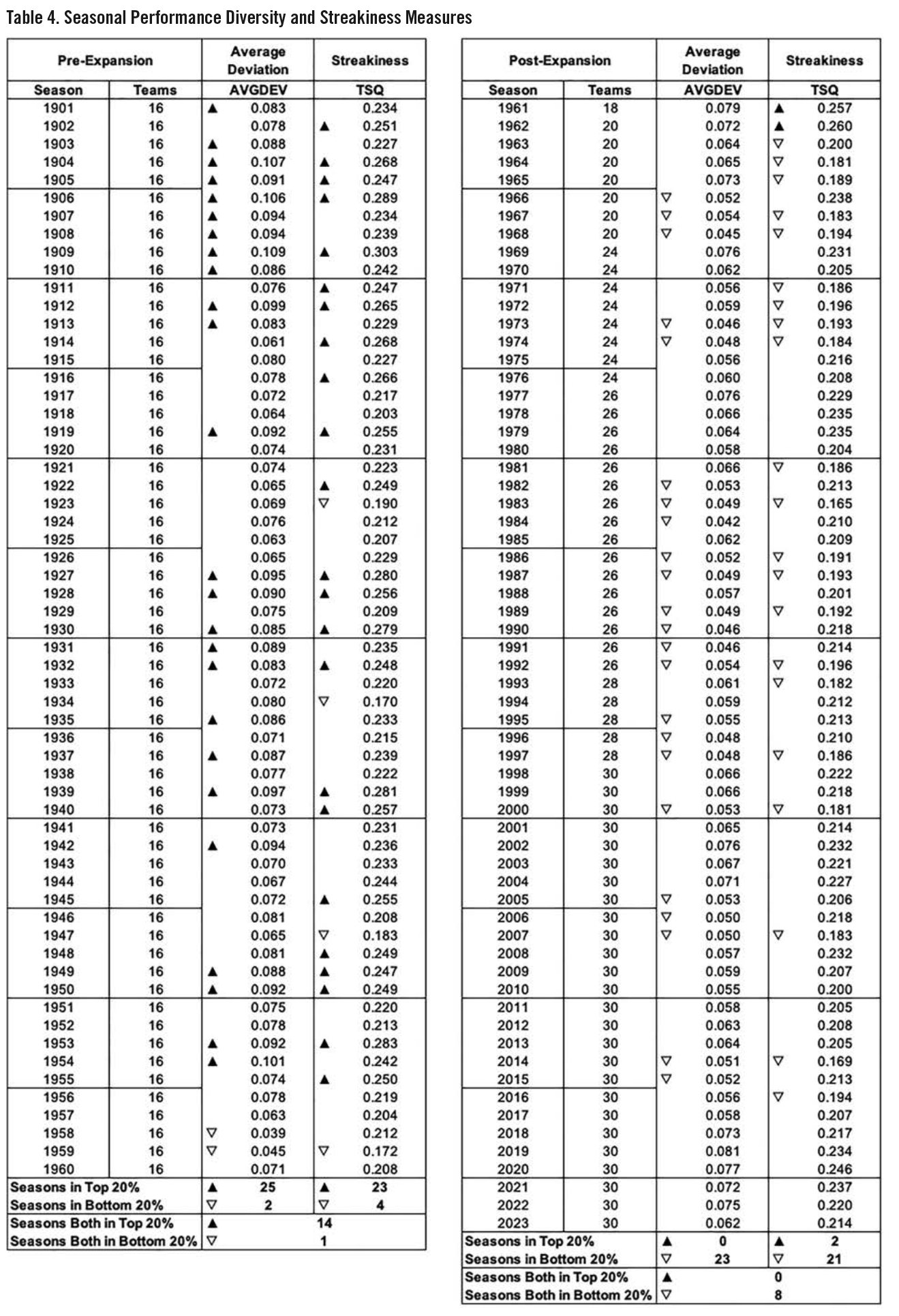
Table 5 depicts a statistical summary of the seasonal values of AVGDEV and TSQ from Table 4.

COMPARATIVE ANALYSIS: PREDICTIONS VS. ACTUALS
Seasonal streaks are constrained to a single season for a single team. The number of teams has ranged from a low of 16 in 1901–60 to the current high of 30. Each current franchise that existed in 1901 has played 123 seasons through 2023. Each season constitutes one of their 123 team-seasons. The 1998 expansion Tampa Bay Rays and Arizona Diamondbacks have played 26 team-seasons. There has been a total of 2,646 team-seasons since 1901.
Predicting Seasonal Streaks. It has been shown that higher performance diversities lead to more total streaks. Performance Diversity (PD) measures the absolute difference between a team’s winning average (PW), expressed as a three digit decimal number between .000 and 1.000, and .500. The more a team’s winning average deviates from .500 the greater the team’s performance diversity, as demonstrated back in Figure 4. Figure 9 is a snapshot of two Excel tables (aka Model) that implement the expected streak equations to calculate total streaks by streak length. Values for PW (or PD) and the number of games (or decisions) are entered into the cells highlighted in black. PL need not be entered; it is calculated from PW.
Two views of the Model are shown: one used for Team-Season streaks and the other for Global Streaks. The calculations implemented by each version are identical. Both versions are shown to illustrate that winning, losing streaks, and total streaks are predicted by the Team-Season approach when winning average, PW, and Games Played are the inputs. A PW less than .500 will result in more expected loss streaks than win streaks. The example shown is the 1919 Philadelphia Athletics, the team with the single highest actual LSQ, who finished with a record of 36–104, PW=.257. The Model predicts eight losing streaks and an LSQ of .457. Results were streakier than predicted with 12 losing streaks (5, 6, 5, 6, 6, 6, 8, 6, 9, 5, 8, 5) and an LSQ of .721 (75/104). As will be revealed later, the summation of all 2646 team-seasonal predictions is highly accurate.

The Global approach is used to evaluate streaks for an aggregate of team-seasons, using an averaged PD and the total number of decisions for the appropriate team-seasons. Win and loss streaks are not applicable, only the total streak parameters ETSG and ETSGSL are relevant. Figure 9 shows that 163 total streaks were expected in 2023 based on a seasonal PD of 0.562. Actual streaks totaled 159, with 80 winning and 79 losing streaks of at least five games.
Let’s predict the expected total number of seasonal streaks, by streak length, since 1901, using three distinct approaches: Global, Seasonal, and Team-Seasonal. Figure 10 outlines the methodology for each approach.

Global Prediction.The Global Prediction method calculates the average of the 2,646 team-seasonal PDs. The Model predicts 14,002 total expected streaks, Table 6, using a PD value of .5669 and 411,868 global decisions. Streaks are rounded to the nearest whole number.
Seasonal Prediction.The Seasonal Prediction method parses the 2,646 team-seasons into the 123 seasons. The average PD is calculated, and the total number of decisions summed for each season. The average PD and the number total decisions for each season is input to an instance of the Model yielding the predicted number of streaks for each season by streak length. To efficiently process 123 seasonal data pairs, an Excel macro to implement the expected streak Model was developed. The power of the macro was crucial to this prediction and even more important when evaluating the Model 2,646 times during the Team-Season approach.
The number of streaks for each streak length is summed for the 123 seasons to yield 14,042 total expected streaks, Table 7.
Table 8 shows the results of the seasonal streak prediction season by season.
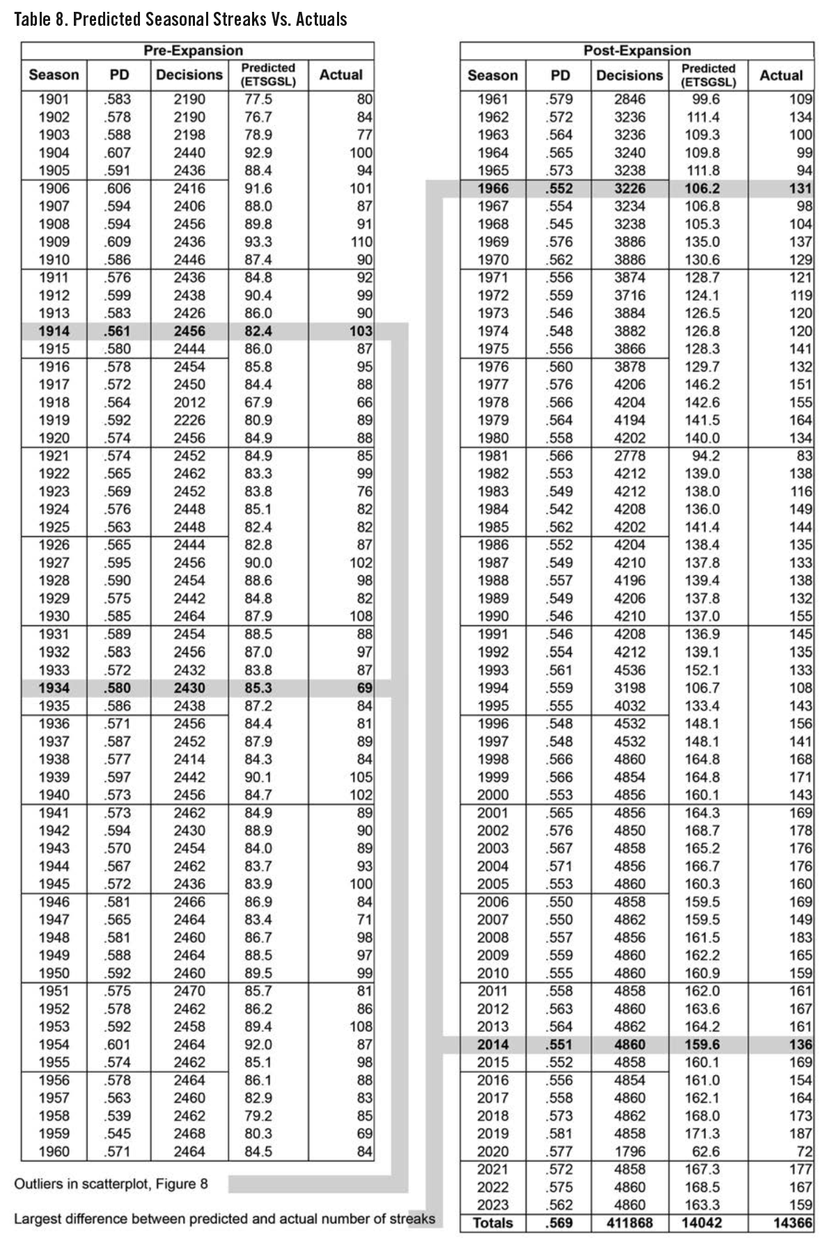
Team-Season Prediction. The Team-Season Prediction method is similar to the Seasonal method. The most critical difference is that it uses the winning average, and not the performance diversity, for each team and each season. This allows both winning and losing streaks to be calculated for each team-season. The PW and decisions for each team-season is input to an instance of the Model yielding the predicted number of both winning and losing streaks for each team-season by streak length. The number of streaks for each streak length and decision type is then summed for the 2,646 team-seasons to yield the expected streak totals as shown in Table 9.
Note that there are more losing streaks than winning streaks for all streak lengths from eight through 22 with only two exceptions (where they are equal), streak lengths 19 and 21. However, winning streaks exceed losing streaks for streak lengths from five through seven. This will become more noteworthy when we compare predictions to actuals and seek to understand the underlying mathematics. Stay tuned.
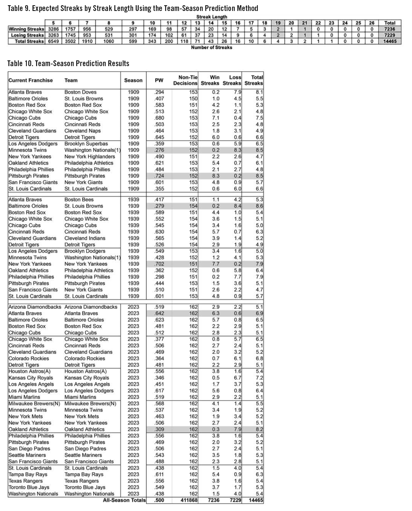
Table 10 displays a few selected season results from the team-season prediction. Highlighted entries represent high winning averages resulting in more streak wins than losses during each season and the reverse for low winning averages.
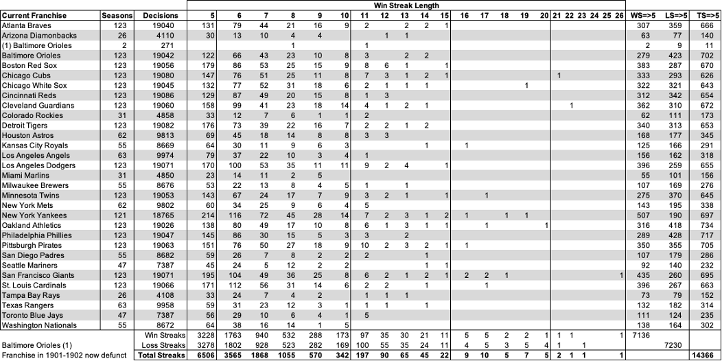
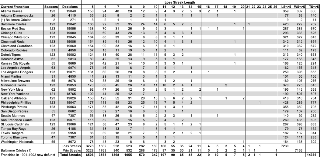
Actual Seasonal Streaks. Actual seasonal streaks are deduced from the encoded data set using filters and functions in Excel. Table 11 breaks down 14,366 actual seasonal winning and losing streaks by franchise and total streaks by streak length.
Global Comparison of Streak Predictions to Actuals. Figure 11 plots the predicted number of seasonal streaks for all three prediction methods along with the actual streaks by streak length for all 411,868 decisions. This is a logarithmic plot. Each horizontal line represents a 10 times difference. The separation between 1 and 10 are all single-digit number of streaks.
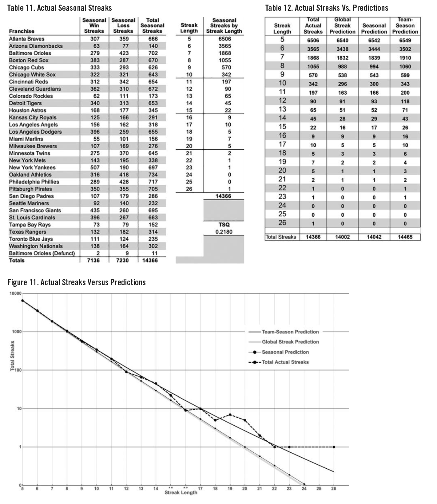
Global and Seasonal predictions are virtually indistinguishable. The Team-Seasonal prediction is very accurate. Actual streaks, 14,366, differ from the Team-Season prediction, 14,465, by only 99 (0.68%). Note that the Team-Season prediction has a slight upward curve.
Figure 12 plots actual win and loss streaks by streak length against the Team-Season predictions.
It is clear that there are more loss streaks (dashed line) than win streaks (solid line), both actual (dark lines) and prediction (gray lines), for streak lengths beginning at 11.

Understanding the Difference Between the Team-Season and Seasonal Analysis. On Figure 11, the Seasonal Prediction appears to be linear, but the Team-Season Prediction has a slight upward bend that more accurately matches the actual number of total streaks. Figure 10 shows that both these prediction methods utilize the Model multiple times and then sum the output expected streaks by streak length. The Seasonal method utilizes 123 instances of the Model (one per season). The Team-Seasonal method utilizes 2,646 instances of the Model (one per team-season).
When the PDs of the individual teams are averaged to derive the seasonal PD, higher and lower individual team PDs get suppressed. Example, in 2010, the Tigers and the Athletics each had a PD of .500 (lowest) and the Pirates and Mariners had PDs of .648 and .623 (the highest two), respectively. The seasonal PD for 2010 is .555 (the average). The Seasonal PDs range from a low of .539 (1958) to a high of .609 (1909). Team-Season PDs range from a low of .500 to a high of .765 (by the 1916 Philadelphia A’s).
Figure 13 (opposite), shows the distribution of the PD values input to the Model for the two prediction methods. This is a bin plot; values are counted and placed in bins. The data point 269 on the Team-Season plot at .625 indicates that 269 of the 2,646 PDs are in the range from .601 to .625.
The shaded area of Figure 13 shows that 484 of the 2,646 PD instances (18.1%) for the Team-Season prediction exceed the maximum PD input to the Model for the Seasonal prediction of .609.
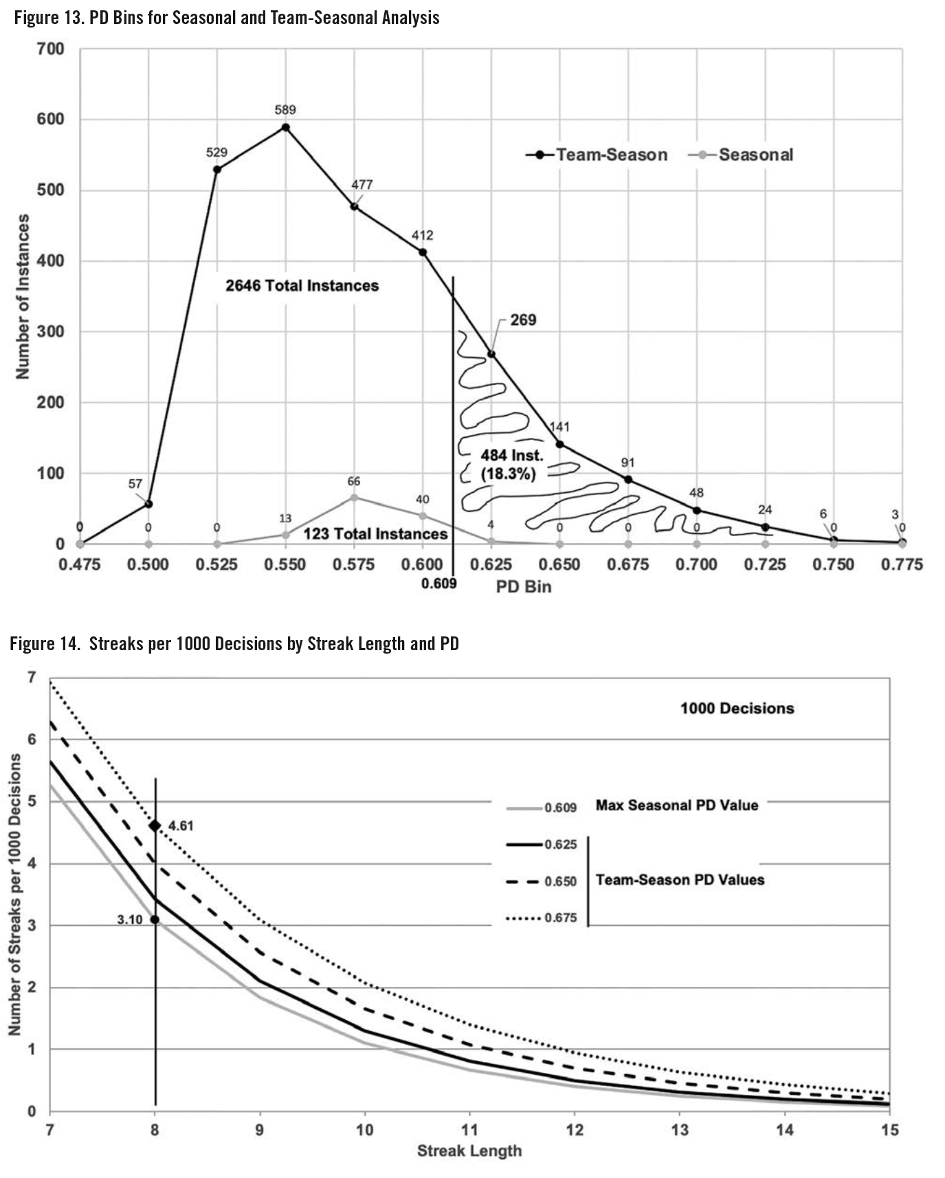
Figure 14 displays the expected number of streaks (between lengths 7 and 15) in 1,000 decisions for several PDs used in the Team-Seasonal Prediction (.625, .650, and .675) and .609 the highest PD in the Seasonal Prediction.
Figure 15 plots the streak differences (per 1,000 decisions) between PD Team-Seasonal values 0.625 and .650) and the highest PD value (.609) used in the Seasonal Analysis. Clearly the Team-Seasonal prediction yields more long length streaks. Hence, the greater the number of long streaks in the Team-Seasonal prediction in Figure 11.

Seasonal Comparison of Streak Predictions to Actuals. Figure 16 plots the predicted number of seasonal streaks against actuals taken from Table 8. Very good correlation can be seen in spite of the relatively small seasonal decision space, less than or equal to 4,860 decisions, 30 teams playing 162 games.
Actual streaks in 1966 exceeded predictions by the largest amount, 131 to 108.3. Actual streaks lagged predictions by the greatest amount in 2014, 136 to 161.9.2
Figure 17 provides a more rigorous view of the accuracy of the seasonal streak predictions. It plots the ratio of Actual Streaks to Predicted Streaks, ETSGSL. Actuals differed from predictions by more than 15% in only nine of the 123 seasons (7.3%). Only three seasons deviated by more than 20%: 1914 and 1966 by +21% and 1934 by -22%. As expected, 1914 and 1934 are the noteworthy outliers on the scatterplot in Figure 8.

CONCLUSIONS
The primary goals in writing this research paper were to:
- explore an area of baseball’s recorded history using a novel analysis technique;
- satisfy my curiosity and fascination about baseball winning and losing streaks;
- present results that would be easily understood by an average, interested baseball fan.
I grouped my analysis into three main areas:
- Mathematical theory and equations to predict streaks verified by simulations;
- Analysis of the correlation between streakiness and performance diversity;
- Comparative analysis between streak predictions and actual results.
I posed two questions: How often and when do streaks occur? Do they follow any predictable patterns?
Streak Prediction. Streak prediction in the long run is embodied by algebraic expressions based on streak length (S), winning average (PW), performance diversity (PD), and the number of the games (N)/decisions (D) being analyzed. (See equations 8b, 9b, and 10b which were confirmed by simulations, Figure 3).
This analysis cannot predict, however, when a streak is likely to start or end, only how often they are likely to occur, given a team’s winning average (PW).
Correlation of Streakiness and Performance Diversity. A new metric, Total Streak Quotient (TSQ), was defined to measure and quantify seasonal streakiness. TSQ is defined as Streak Wins (SW) plus Streak Losses (SL) divided by Decisions (D). SW (or SL) is number of wins (or losses) during a season that are part of winning (or losing) streaks of five or more games. Seasonal performance diversity was quantified by Average Deviation (AVGDEV) which is defined as the average of the absolute deviations of the winning average of all teams in the league from the mean for a given season (which is always .500).
Season by season comparison of TSQ and AVGDEV shows noteworthy correlation as evidenced by the scatterplot of Figure 8. Greater performance diversity (higher AVGDEV) leads to greater streakiness (higher TSQ) and more total streaks.
Comparison of Streak Actuals and Predictions. The total number of streaks by streak length in the global sense is quite predictable, as evidenced by Figure 11 and 12. The following critical components were developed to investigate winning and losing streaks:
- A proprietary conversion scheme to replace each win, loss, and tie in baseball history since 1901 with an encoded numerical value that facilitates streak data extraction;
- An easily understood test sequence slide model used to develop the expected streak equations (8b, 9b, and 10b);
- An Excel Macro Model to repeatedly evaluate the expected streak equations and predict streaks on a team-season and seasonal basis;
- A detailed visualization of the mathematical relationship between performance diversity and streaks.
The total number of streaks for the league in shorter seasonal runs is still predictable within slight margins, as evidenced by Figures 16 and 17. The specific teams that own the streaks during a given season are not necessarily predictable. However, it is obvious that better teams have more winning streaks than losing streaks, and poorer teams more losing streaks than winning streaks.
Although there are many factors that can give one team an edge, the outcome of any specific baseball game is uncertain. Winners are determined on the field and outcomes can exhilarate and surprise. Some things, however, are undeniable.
- Every (non-tie) game played to completion has only a winner and a loser.
- There are an equal number of wins and losses in the league each season.
- More than 206,000 games have been played.
- Some teams are better than others.
These certainties and the degree to which teams are better or worse than .500 form the basis for the predictability of streaks.
I trust my research has fostered a new understanding of modern baseball’s winning and losing streaks.
ED DENTA is a retired professional engineer and lifelong baseball fanatic. Ed umpired Florida high school baseball for 18 years. Ed combines an analytical background and fervor for history/ statistics to research and author sports-related artifacts. Ed is an active member of the Roush-Lopez Chapter of SABR in the Tampa Bay area.
Notes
1 Baseball Reference and other sites owned by Sports Reference LLC allow the general public to share, export, and use their data as long as they are credited. Game results are also found at Retrosheet.org
2 Seasons 1981 and 1994 were shortened seasons due to work stoppages. 2020 was a 60-game season because of COVID-19 mitigation measures.
APPENDIX
Table A-1. Seasonal Win Streaks by Franchise
(Click image to enlarge)
Table A-2. Seasonal Loss Streaks by Franchise
(Click image to enlarge)
Acronyms
|
Acronym |
Definition |
Description |
|
=> |
greater than or equal to |
|
|
AL |
American League |
|
|
AVGDEV |
Average Deviation |
a metric to evaluate seasonal performance diversity; defined as the average of the absolute deviations of the winning percentage for all teams in the league from the mean (that is always .500) for a given season |
|
BoS |
Beginning of Season |
type of streak where the final five or more non-tie results at the beginning of a season are either all wins or all losses |
|
CD |
Composite Diversity |
a single value of the probability of winning (PW) that is used to predict the combined total numbers of streaks for all baseball seasons; it is calculated by averaging the 123 seasonal PWs that best predict the actual number of total streaks for each season |
|
D |
Decisions |
number of non-tie decisions when evaluating league-wide streaks |
|
DEV |
Deviation |
the difference between a team’s winning percentage (PW) and .500, i.e. .500-PW; it is a negative value when PW is less than .500 |
|
ELS |
Expected Losing Streaks |
expected number of losing streaks for a .500 team for a given streak length S |
|
ELSG |
Expected Losing Streaks Generalized |
expected number of losing streaks for any team for a given streak length S |
|
ELSGS |
Expected Losing Streaks Generalized Summed |
expected number of total losing streaks for any team for all streak lengths |
|
ELSGSL |
Expected Losing Streaks Generalized Summed League-Wide |
expected number of total losing streaks league-wide for all streak lengths |
|
EoS |
End of Season |
type of streak where the final five or more non-tie results at the end of a season are either all wins or all losses |
|
ETS |
Expected Total Streaks |
expected number of total streaks for a .500 team for a given streak length S |
|
ETSG |
Expected Total Streaks Generalized |
expected number of total streaks for any team for a given streak length S |
|
ETSGS |
Expected Total Streaks Generalized Summed |
expected number of total streaks for any team for all streak lengths |
|
ETSGSL |
Expected Total Streaks Generalized Summed League-Wide |
expected number of total streaks league-wide for all streak lengths |
|
EWS |
Expected Winning Streaks |
expected number of winning streaks for a .500 team for a given streak length S |
|
EWSG |
Expected Winning Streaks Generalized |
expected number of winning streaks for any team for a given streak length S |
|
EWSGS |
Expected Winning Streaks Generalized Summed |
expected number of total winning streaks for any team for all streak lengths |
|
EWSGSL |
Expected Winning Streaks Generalized Summed League-Wide |
expected number of total winning streaks league-wide for all streak lengths |
|
IS |
In-Season |
type of streak where five or more non-tie results within a single season are either all wins or all losses; beginning of season (BoS) and end of season (EoS) streaks are also considered in-season (IS) streaks |
|
LLC |
Limited Liability Company |
|
|
LLS |
Longest Losing Streak |
the longest losing streak of the season |
|
LSQ |
Losing Streak Quotient |
Streak Losses (SL) divided by Total Losses (TL) |
|
LWS |
Longest Winning Streak |
the longest winning streak of the season |
|
MLB |
Major League Baseball |
|
|
N |
Number of decisions |
number of decisions when evaluating single-team streaks |
|
NL |
National League |
|
|
NT |
Number of Tests |
number of required tests to evaluate for a given streak length over a given decision sequence; T=N-S+1, where N is the number of decisions evaluated and S is the streak length |
|
PCT |
Percentage |
More specifically, winning percentage; it is calculated by dividing games won by decisions, and expressing the result as a three digit number between 0.000 and 1.000; also, a team’s probability of winning (PW) |
|
PD |
Performance Diversity |
a metric to evaluate seasonal performance diversity for a given team-season; defined as Average Deviation, AVGDEV, plus .500; PD is equal to PCT or PW for teams with a PCT or PW greater than or equal to .500 |
|
PH |
Probability of Heads |
probability of a single fair coin toss coming up heads, 0.5 |
|
PK |
Probability of K coin tosses |
probability of a single fair coin being tossed K times and yielding a specific, sequential result |
|
PL |
Probability of a Loss |
probability of a loss; also, one minus the team’s losing percentage |
|
PT |
Probability of Tails |
probability of a single fair coin toss coming up tails. 0.5 |
|
PW |
Probability of a Win |
probability of a win; also, a team’s winning percentage (PCT) |
|
S |
Streak |
length of a winning or losing streak |
|
SABR |
Society for American Baseball Research |
|
|
SL |
Streak Losses |
number of losses during a season that are part of losing streaks of five or more games |
|
SRL |
Sports Reference LLC |
|
|
ST |
Streak Decisions |
number of decisions during a season that are part of streaks of five or more games |
|
SW |
Streak Wins |
number of wins during a season that are part of winning streaks of five or more games |
|
T |
Tests |
the required length of a test sequence to evaluate for a given streak length over a given game sequence; T=S+2, where S is the streak length |
|
TL |
Total Losses |
total games lost during season |
|
TS |
Test Sequence |
Length of a test sequence |
|
TSQ |
Total Streak Quotient |
a normalized metric to evaluate streakiness; defined as Streak Wins (SW) plus Streak Losses (SL) divided by total non-tie Decisions (D) |
|
TW |
Total Wins |
total games won during season |
|
WA |
Wraparound |
type of streak where the final non-tie result at the end of a season matches the first non-tie result of the succeeding season and the combined consecutive matching results across the two seasons total at least five games |
|
WSQ |
Winning Streak Quotient |
Streak Wins (SW) divided by Total Wins (TW) |
Identities
1/ab=a-b or 1/ab=a-b
By definition, D=2N, when referring to multiple teams
By definition, D=N, when referring to a single team
By definition, ETS=EWS+ELS
By definition, ETSG=EWSG+ELSG
By definition, ETSGS=EWSGS+ELSGS
By definition, ETSGSL=EWSGSL+ELSGSL
By definition, PCT=PW
By definition, PD=AVGDEV+.500
By definition, PH+PT=1
By definition, PW+PL=1
By definition, ST=SW+SL
By definition, T=N-S+1
By definition, TS=S+2