

Is a Major League Hitter Hot or Cold?
This article was written by David D. Marx - Anne C. Marx Scheuerell - Megan Liedtke Tesar
This article was published in Fall 2013 Baseball Research Journal
Many major league baseball games are decided in the final innings or outs of a game. For that reason, it would be beneficial for team managers to know which player on their team has the highest probability of getting on base or getting the game-winning hit. The probability, however, will differ depending on whether the player is hot or cold. The goal of this study is to use hidden Markov models to determine when players are hot or cold and to determine how their batting averages differ between these two states.
INTRODUCTION
The World Series is tied at three games apiece. Going into the decisive seventh game, which players would you prefer to have in the lineup? If it is the bottom of the ninth inning, the score is tied 2–2, and the bases are loaded, do you stick to the lineup or put in a pinch-hitter? This question had to be answered by Bob Brenly, the manager of the Arizona Diamondbacks, in the 2001 World Series against the New York Yankees. Brenly stuck to the lineup, and fortunately for the Diamondbacks, despite his 11 strikeouts and a .231 batting average (6 for 26) in the series, Luis Gonzalez came through with a single to center to win the series.
 Many major league baseball games are decided in the final innings or outs of a game. For that reason, it would be beneficial for team managers to know which player on their team has the highest probability of getting on base or getting the game-winning hit. The probability, however, will differ depending on whether the player is hot or cold. Previous studies have addressed streakiness in hitting (Albert, 2004; Albright, 1993), yet data did not support a pattern of streakiness across all players. The goal of this study is to use hidden Markov models to determine when players are hot or cold and to determine how their batting averages differ between these two states.
MARKOV CHAIN
To understand the concept of a Markov chain, consider the following example. During a seven-day time period, the weather can be observed and classified as sunny, cloudy, or rainy. These three classifications are called the observable states, and the probabilities of moving from one state to another are known. These probabilities, called transition probabilities, are the only parameters in a regular Markov model because the state is directly visible to the observer. In addition, the probability of observing a certain weather condition today is based only on the previous day’s weather. In addition, the probability of observing a certain weather condition today is based only on the previous day’s weather rather than the observed weather state two, three, four, etc. days ago. When these conditions are satisfied, the process can be described as a Markov chain.
By definition, a Markov chain, denoted by {Xn}, is a process with a countable number of states and discrete units of time t = (0, 1, 2 …, n) such that at each time the system is in exactly one of the states. Furthermore, a Markov chain contains known transition probabilities. Following the notation used by Karlin (1969, pp. 27), the transition probability of being in state j at time period n+1 given that the process is in state i at time n is denoted by:
Pij = P(Xn+1 = j | Xn = i)
As mentioned above, these transition probabilities rely exclusively on the current state of the process. Therefore, knowledge regarding its past behavior does not influence the probability of any future behavior. In more formal terms,
P(Xn+1 | X1, X2, …, Xn) = P(Xn+1 | Xn)
where the value of Xn is the state at time t = n. In a Markov chain, the probability of the system beginning in each of the states must also be defined. Let p0i denote this transition probability from the beginning state (state 0) to state i or the probability of starting in state i.
Now any sequence from a Markov chain can be written as X1, X2,X3, X4, . . . Xn, and the probability of this sequence is as follows:
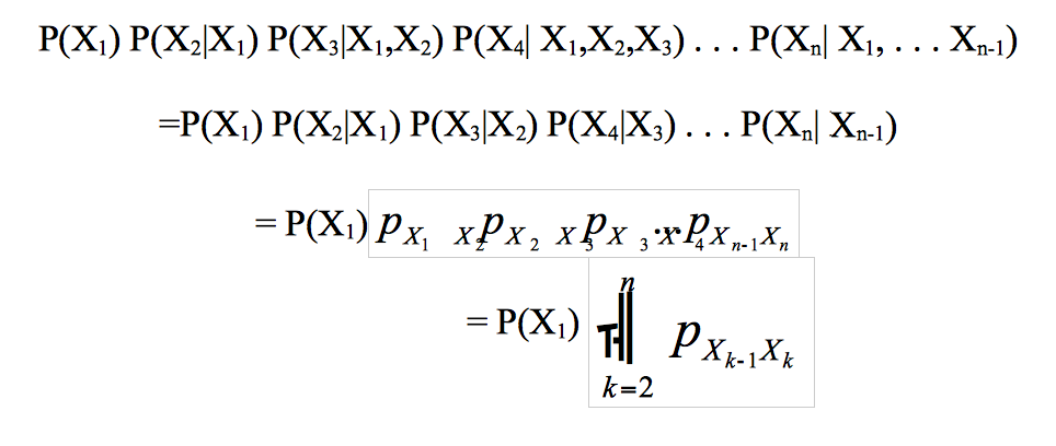
This proof is based on the definition of a conditional probability and by applying the property that probability of each state depends only on value of preceding state.
In this study, a Markov chain is used to model the hitting of major league baseball players over the course of a season. The Markov chain has two possible states (hot and cold), and the transition probabilities model the chance that a player will transition from one type of hitting to another.
Will this chain satisfy the Markov property? In other words, is the future hitting type dependent only on the current hitting type? It is clear that previous states might lend some information about the next transition. For example, if the previous few states are cold, the batter may be in a series against a team with a tough pitching staff, and it will be more likely for the next state to be a cold. However, this situation might be uncommon because of the large amount of variation in throwing style among pitchers. Although thinking about whether or not this chain satisfies the Markov property is important, a model can still be useful even if it is not exact.
HIDDEN MARKOV MODEL
According to Durbin, Eddy, Krogh, and Mitchison (1998), a hidden Markov model (HMM) is a “probabilistic model for sequences of symbols” (p. 46). Unlike a regular Markov model, the state is not directly visible. However, variables influenced by the state are visible, and the challenge is to determine the hidden states from an observable variable.
In major league baseball, the type of hitting is not directly visible. Thus, we will be using a hidden Markov model with the number of successful plate appearances per game as the visible variable.
The three main components of a HMM include an initial distribution, an emission matrix, and a transition matrix. The initial distribution defines the probability of the model being in each hidden state at time t = 0. The emission matrix contains the probabilities of each observable variable given that the model is in a particular hidden state, denoted
ei(b) = P(xk=b|Xk=i)
Lastly, the transition matrix contains the probabilities of being in each hidden state at time t = n given the hidden state at time t = n-1.
DATA
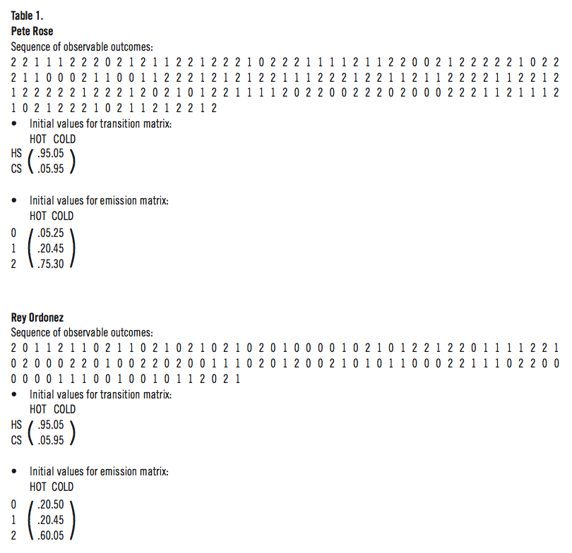
This study is based on detailed information about each player’s plate appearances over the course of their career (Baseball-Reference.com, Forman, 2000). For this analysis, the 1978 season of Pete Rose will be contrasted to the 1997 season of Rey Ordonez. During the 1978 season, Rose had 731 plate appearances and at least one hit in 44 consecutive games. In 1997 Rey Ordonez had 391 plate appearances and went 37 consecutive plate appearances without a hit.
Using the outcome of each plate appearance, the number of successful plate appearances per game was calculated for each player. The criterion for a successful plate appearance was reaching base on a single, double, triple, home run, base on balls, intentional base on balls, or by being hit by pitch. Never reaching base and reaching base on an error or a fielder’s choice were considered unsuccessful plate appearances. Using the number of successful plate appearances in a game, three observable states were formed. The first state is defined as 0 successful plate appearances in a game, the second state is 1 successful plate appearance, and the third state is greater than or equal to 2 successful plate appearances in a game.
EXAMPLE
During each major league baseball game, there is a certain chance that each player will have 0, 1, or “2 or more” successful plate appearances. The probability of each observable variable is determined exclusively by the type of hitting the player is in. The two types of hitting represent our hidden states and will be denoted by “HOT” for a hot and “COLD” for a cold. No definite information about the hitting type is known, but we will try to determine the type based on the number of successful plate appearances per game.
The initial transition matrix was created based on knowledge that one game of plate appearances does not constitute a hitting type. For that reason, a probability of .95 was chosen for staying within a state and .05 was chosen for the probability of changing states. The starting values for the emission matrices are based on the percentage of times each observable variable appears in the sequence. The average of the hot probability and cold probability for each observable outcome is approximately equal to the percentage of times it occurs in the sequence. The sequence of observable outcomes and the initial transition and emission matrices for Rose and Ordonez are given in Table 1.
(Click image to enlarge)
MODELING METHOD
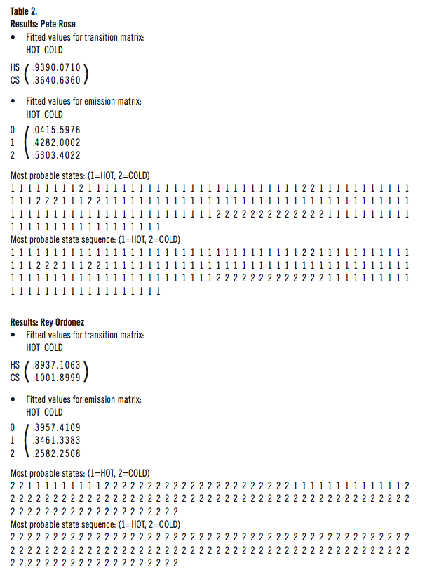
Three functions in the hmm.discnp package of R were utilized in this study (Turner, 2006). First, a hidden Markov model was fit to the sequence of successful plate appearances using the Expectation-Maximization algorithm. This algorithm finds the most likely set of transition and emission matrices based on the data and by using the initial values of the matrices as the starting point. The most probable hidden state (HOT and COLD) underlying each observation was then found based on the sequence and the resulting hidden Markov model. Finally, the Viterbi algorithm (Viterbi, 1967) was used to determine the most likely sequence of hidden states (HOT and COLD) that could have generated the sequence. It is important to realize that the sequence of most probable states will not in general be the most likely sequence of states. The results from these three functions are given in Table 2.
(Click image to enlarge)
INTERPRETATION OF RESULTS
 There is a large difference between the hot and cold emission probabilities for Pete Rose. He had approximately a 4% chance of having 0 successful plate appearances during a game, a 43% chance of having 1 successful plate appearance, and a 53% chance of having 2 or more successful plate appearances given he was hot. However, he had approximately a 60% chance of having 0 successful plate appearances, a 0% chance of having 1 successful plate appearance, and a 40% chance of having 2 or more successful plate appearances given he was cold. Furthermore, the probability of staying in a hot is .9390 while the probability of staying in a cold is .6360.
Based on the resulting most probable states and most probable sequence of states, Rose was hot for the majority of the 1978 season. These results are not shocking because it was one of his most successful hitting seasons, although not one of his most successful total offensive seasons. The longest he was cold of the season lasted 13 games. In this 13 game stretch, there were 7 games when he had 0 successful plate appearances.
On the other hand, there is a small difference in the emission probabilities for Ordonez indicating that the model failed to find two different states. He had approximately a 40% chance of having 0 successful plate appearances during a game, a 35% chance of having 1 successful plate appearance, and a 26% chance of having 2 or more successful plate appearances given he was hot. In addition, he had approximately a 41% chance of having 0 successful plate appearances, a 34% chance of having 1 successful plate appearance, and a 25% chance of having 2 or more successful plate appearances given he was cold. Furthermore, the probability of staying in a hot is .8937 while the probability of staying in a cold is .8999.
Based on the most probable sequence of states, Ordonez was in a cold state for the entire 1997 season. However, the most probable was a hot state for 13 consecutive games. This occurred when Ordonez successfully reached base in 12 of the 13 games.
CONCLUSION
Going into Game Seven of the World Series, should the manager put Pete Rose or Rey Ordonez in the lineup? It depends! Based on the model, the probability that Rose will have 0 successful plate appearances given that he came into the game in a cold state is,
P(0n+1|COLDn) = 0.64(0.60) + 0.36(0.04) = 0.4.
Likewise, for Ordonez,
P(0n+1|COLDn) = 0.90(0.41) + 0.10(0.40) = 0.4.
Therefore, if both players come into the game in a cold state, they have the same probability of having an unsuccessful game.
However, based on the model, the probability that Rose will have 0 successful plate appearances given that he came into the game in a hot state is,
P(0n+1|HOTn) = 0.94(0.04) + 0.07(0.60) = 0.08.
Likewise, for Ordonez,
P(0n+1|HOTn) = 0.89(0.40) + 0.11(0.41) = 0.40.
Therefore, if Rose is in a hot state, he has a much lower probability of having an unsuccessful game and he is the player you want in the lineup.
MEGAN LIEDTKE TESAR is taking time away from her career as a statistics professor to be at home with her son Eli. She received her master’s degree and Ph.D. in Statistics from the University of Nebraska-Lincoln. She was also a postseason-honor-winning college softball player and has great respect for the catcher position.
ANNE C. MARX is Assistant Professor of Sport Management at Loras College in Dubuque, Iowa. She earned her Master’s Degree from Arizona State University and doctorate degree from the University of Arkansas. She is an avid athlete and can be seen in the evenings playing baseball with her son, Adam, in the back yard.
DAVID B. MARX is Professor of Statistics at the University of Nebraska in Lincoln, Nebraska. He works in the area of spatial statistics as well as in sports statistics. His Ph.D. is from the University of Kentucky and he was previously employed at the University of Arizona and University of Arkansas. He is a member of the American Statistical Association’s section of Statistics in Sports.
REFERENCES
Albert, J. (2008). Streaky hitting in baseball. Journal of Quantitative Analysis in Sports, 4(1). Retrieved August 2013 from http://www.stat.berkeley.edu/~aldous/157/Papers/albert_streaky.pdf.
Albright, S. (1993). A statistical analysis of hitting streaks in baseball. Journal of the American Statistical Association, 88, 1,175–83.
Durbin, R., Eddy, S., Krogh, A., & Mitchison, G. (1998). Biological Sequence Analysis, Cambridge: Cambridge University Press.
Forman, S. L. (2000). Baseball-Reference.com–Major League StatistiCOLD and Information, Retrieved June, 2007 from http://www.baseball-reference.com.
Karlin, S. (1969). A First Course in Stochastic Processes, New York, NY: Academic Press, Inc.
Turner, R. (2006). The hmm.discnp Package, Retrieved June 2007 from http://www.math.unb.ca/~rolf.
Viterbi, A. J. (1967). Error bounds for convolutional codes and an asymptotically optimum decoding algorithm. IEEE Transactions on Information Theory 13 (2), 260–69