Luck, Skill, and Head-to-Head Competition in Major League Baseball

In this article I deal with two issues: the relationship between luck and skill in Major League Baseball and the role of matchups between teams in season competition. The former issue is dealt with to assess the significance of the latter.

It is generally felt that both skill and luck are factors in determining success or failure. Being in the right place at the right time is considered a matter of luck. Preparation and ability are acknowledged to be skill factors. What constitutes skill and what constitutes luck in baseball? How do we assess the relative contribution of luck or skill in determining game outcome? The spectacular catch by Willie Mays in game one of the 1954 World Series is a prime example of superb skillful performance. The bad hop over Fred Lindstrom’s head in the 1924 World Series is a clear example of extremely bad luck. On the other hand, how do we evaluate the ground ball off of Billy Loes’s leg in the 1952 World Series that he said was lost in the sun? All of these illustrate key events in determining game outcomes. The problem to be addressed is finding out the relative contribution of luck or skill to victory or defeat.

In order to solve the problem, we must consider identifying the variables that are related to game outcome. Insofar as we can identify performance measures that relate to team outcome, we have potential indicators of skill. After such measures are applied to predict outcomes, we can observe how much variability in outcomes remains. Such variability may result from in part luck and in part skill. Here is where it is important to be able to assess how much variability in performance would occur if only randomness or “chance” (which we call luck) determines the outcome. My approach includes such an assessment, as we will see.

There is a long history of trying to find the factors that account for team success, to specify how they work, and separate them from luck. Perhaps the most notable is Bill James’s Pythagorean expectation, named for its resemblance to the well known Pythagorean Theorem.¹ His basic formula is

       rs²       
(rs² + ra²)

where rs is runs scored and ra is runs allowed. Runs scored and runs allowed are two very direct measures of team effectiveness that are combined in the formula for predicting team success. The formula is used to estimate how many games a team “should” have won, with any difference between actual and estimated values attributed to luck. The rationale for the exponent 2 is based upon the use of the ratio rs/ra as a measure of “team quality,” with reciprocal of the ratio used as the measure for a generalized opponent. However, searches were made to find an exponent that better predicted winning percentage (for example, the work of Clay Davenport and Keith Woolner,² and David Smith³). Insofar as values are based on empirical fits, they do not represent a theoretical basis for explaining the process.

Since systematic differences between actual and expected winning percentages using the formula occur (e.g., big winners “should” have won less, and big losers “should” have won more), other measures that could relate to team performance have been introduced into the formula. After all, runs may be scored as a result of luck as well as skill. Variables such as on base percentage and earned run average may help get around the luck factor. Having a measure of the possible effect of a luck factor may help us.

Using a different approach, Pete Palmer examined the variability between teams in win records over many seasons and compared it with what would be expected if teams were all equal in skill, and all variability between teams was a matter of luck.⁴ Palmer concluded that since 1971 the contribution of luck and skill have become nearly equal. The apparent decreasing relative contribution of skill may reflect a trend toward parity. Luck would then play an increasing role in determining outcomes. I deal with this a little later and consider changes in the game other than increased parity.

THE HEAD-TO-HEAD PERFORMANCE VARIABLE

I have looked at the possibility that another factor related to skill contributes to differences between teams in outcomes: head-to-head competition. John Richards has developed an approach that predicts head-to-head outcome probabilities using relative overall season success of the two competing teams.⁵ However, I show that a team may produce significantly more or fewer wins against a given team than would be expected by its overall season performance. Such a result may well be attributable to unique differences between teams in terms of relative strengths and weaknesses. I test the hypothesis that head-to-head performance variation may be something more than chance variation over a season.

A season for a given team may be considered as a set of “mini seasons” consisting of the season’s series for two teams in contention for the pennant. In this light we may look at a team’s win record as the sum total of average total season performance and performance over and above (or below) its average total season performance against certain teams. If the hypothesized impact of specific factors related to particular team matchups is found, another variable may be added to total season performance. Insofar as this factor is identified, the contribution of the skill factor is increased, and the relative contribution of luck is thereby decreased. Here is where the assessment of the skill-luck relationship becomes tricky. Although, as we will see, we may be able to calculate the variation that would exist if only pure luck determines outcomes, we can always potentially find different performance variables associated with skill that increase the contribution of the skill factor. Hence, the contribution may always increase relative to luck.

To illustrate how assessment of the head-to-head factors would work, Figure 1 shows the season win record of the Chicago White Sox against each of its seven opponents in the 1954 season. The 1954 White Sox present a clear example of overall superior performance save for unusual difficulty in beating the Yankees. Their general pattern of victories against other opponents suggests some head-to-head effects. The seven opponents are denoted in the chart in positions corresponding to the number of White Sox victories against them in their season series. The White Sox won 94 games for an average of 13.43 wins per opponent.

 

 

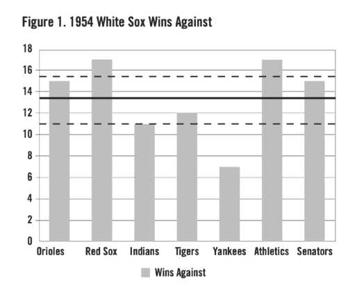
We would expect the average victories per opponent to converge to that value over many repetitions of the 1954 season, assuming the White Sox performance was independent of opponent played, and luck was the only factor causing variation from that average. It is, of course, assumed the White Sox remain a .610 team over all replications. The solid horizontal line from the vertical axis reflects the chance baseline value of 13.43 games. The distances from this line may represent variation attributable to either luck, skill, or some combination of the two.

To make the appropriate assessment, we need a measure of how much variation— such as shown in Figure 1—is attributable to pure random variation or luck. We also need a comparable measure of actual variation. Using Figure 1 as an example, we can find the average of the squared differences between number of White Sox victories against each of the seven teams and the mean of 13.43. The resulting value is 11.39. To generalize, we can find a measure of variability between teams for a season by subtracting mean number of victories for all teams from the number of victories for each team, and averaging the resulting squared differences for all teams. The resulting value is called the variance, which we will see has important properties.

A measure of the variability expected if only luck determines outcomes can be computed using the binomial distribution. The binomial distribution is produced by the sum of a number of independent observations on a variable that assumes two possible values: zero or one. In our example, one stands for victory and zero for defeat. For a large number of such observations, the binomial distribution approximates the normal bell-shaped distribution. Suppose p is the probability of victory for a team, and hence (1−p) the defeat probability. The expected number of victories for a team in a season is then number of games × p.

In the White Sox example, the best estimate of the value is 154 × .610 victories for their season total. If luck dominates, p = .50. In a 162-game season, the expected number of wins for all teams is then 162 × .50 = 81. The variance for a binomial distribution is number of observations × p × (1−p). In our White Sox example, the expected variance of White Sox victories in 22 games against a given opponent if only chance variation from their usual level determines outcome is 22 × .61 × .39 which equals 5.23.

Although the variance has analytic advantages, the square root of the variance, the standard deviation, produces a value in terms of games, which allows for comparisons of interest. The standard deviation in our example is 2.29. The dashed lines above and below the horizontal line in Figure 1 define a band between + and − one standard deviation from the 13.43 mean. In the bell-shaped normal distribution it is expected that values would occur about 68% of the time in this band. In this case, with Cleveland just outside the band, only three of seven teams show results that fell within the range expected by luck alone, which suggests something more than luck might be at work.

So far we have some measure of the independent effect of the head-to-head variable, insofar as variation from the average performance of a given team is measured independently of variation between teams. However, we have neglected to account for the impact of the difference between two teams in overall season performance upon the relative success in matchups between those two teams. Returning to the 1954 White Sox example, the White Sox won 17 of their 22 games against the Red Sox, 3.57 more games above the season average number of wins per opponent. However, the White Sox won 13 more games than did the Red Sox against the other six teams in the league. Dividing by six shows that on average the White Sox beat each of the other six teams in the league 2.17 times more often than did the Red Sox. Thus, 2.17 of the White Sox victories over the Red Sox could be attributed to overall superiority, and the remainder to unique factors related to the head-to-head matchup. The 3.57 games above the per-team average is reduced accordingly to produce a measure of the head-to-head factor for the two teams.

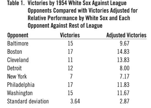
As another example, consider the season series between the Yankees and the White Sox. The White Sox record against the six American League teams other than the Yankees was 87 victories and 45 losses, while the Yankees were 88 and 44 against the same six teams. Thus, the White Sox won one fewer games that did the Yankees against the rest of the league. This means that they averaged .17 fewer victories against each of the other teams than did the Yankees. This difference is a measure of general superiority of the Yankees over the White Sox, and the White Sox would be expected to lose on average .17 games more games than the Yankees against common opponents on the basis of overall team strength. The necessary adjustment would be to add .17 to the White Sox victory total of seven for their season series to reflect a compensating head-to-head factor. We note that making adjustments to victory totals is equivalent to making adjustments to deviations from the per-opponent average in terms of calculating a variance attributable to the head-to-head factor. Table 1 shows the White Sox victories against the seven other teams together with victory values corrected as above. Standard deviations of corrected and uncorrected values are shown for comparison.

 

 

LUCK, SKILL, and HEAD-TO-HEAD PERFORMANCE PRIOR TO 1969

I performed an analysis to assess the relative contribution of overall team performance, head-to-head competition, and the luck factor to variability in team performance. Table 2 shows average standard deviations by decades for total season team performance for each league from 1900 to 1968, the last year before divisional play was introduced. Standard deviations for head-to-head contributions are based on the adjustments for two competing teams differences in victories against the league. I examine the reasons for considering seasons after that separately later.

 

 

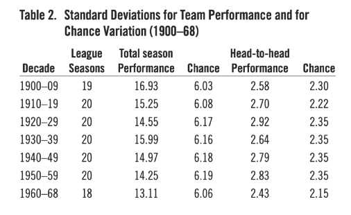
A measure that takes advantage of the additive nature of variances and sums of squared differences was used to calculate the variability attributable to head-to-head matchups. In general, the variance of a sum of independent variables is equal to the sum of their variances. The same cannot be said of standard deviations. It is possible to total the sum of squared differences, such as found in the White Sox example, over all teams in a league for a season. If we use an appropriate denominator for the sum, we get an unbiased estimate of a variance for the league season. The additive nature of variances makes it possible to estimate the relative contribution of head-to-head matchups in a way not possible for standard deviations. The measure corrects for overall team victories for each team, and hence is independent of the variance of overall team victories. It will later be used in a technique called the analysis of variance when other comparisons are made. Table 2 shows the average square roots of the values for each decade. These function as the mean standard deviations for head-to-head contributions. Standard deviations expected for pure luck are also shown for both the total season and head-to-head factors. Results showed a tendency for contribution of total season performance to be much greater than that of head-to-head matchups. I return to these results after considering the data for the era of divisional play.

Palmer noted a tendency for the relative contribution of the skill factor to decline after 1970. This coincided with the introduction of the divisional structure in each league. In the post-1968 era, each team within a division plays every other team in its division an equal number of times. Each team in one division plays each team in the other division an equal number of times, although usually less often than teams in its own division. The intra-divisional setup imposes the same constraints upon the schedule as was true in the pre-divisional era, where total victories must equal total defeats. This constraint does not exist in extra-divisional play. As an extreme example, all teams in one division might win all their games with all teams in the other division.

 

 

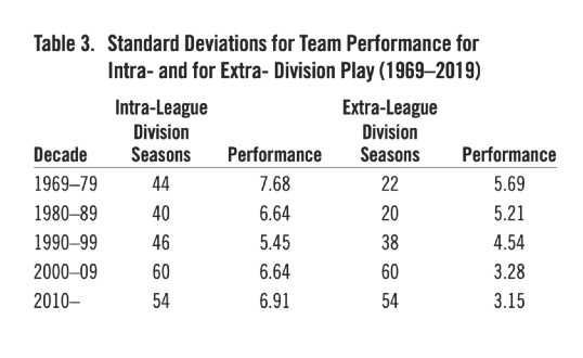
The comparison between intra- and extra-divisional play reflects an important property of variances relevant to assessing performance factors in this situation.⁶ Table 3 demonstrates the clear difference between intra- and extra-divisional play in variability of team records with intra-divisional standard deviations averaging about 1.5 greater than extra-divisional values. Variances related to each other as those in this case can always be expected to show the relationships found. Each extra-division standard deviation was based on a season’s competition between two divisions. The 1994 season was not included in the analysis, because the abbreviated season resulted in very large variations in number of games in head-to-head series that made meaningful analysis not feasible.

Most seasons featuring divisional play have schedules in which more games are played within a division than are played between two divisions. Hence, it is possible that intra-division overall variances for teams are merely larger because of this difference. I found that for the 93 cases in the two-division period in which more intra-division than extra-division games were played, the intra-division and extra-division variances were 59.44 and 32.93 respectively; for the 51 cases in which there were more extra-division games, the intra-division and extra division variances were 45.89 and 32.16 respectively. Thus, number of games within a division could not account for the observed differences in variances. The dynamic of an intra-division balanced schedule seems the most comparable to that for the pre-1969 season schedule. Since both intra- and extra-divisional records figure into the overall performance variance, the variance of overall team victories after 1968 would tend to give a lower estimate of the performance factor relative to that of pre-1969. Thus, intra-division performance should provide the most appropriate measure in making comparisons to pre-1969 performance.

A problem with using intra-divisional results stems from the fact that the smaller intra-division schedule relative to that for the full earlier seasons results in an intrinsically lower performance variance because of a smaller range of possible values. This problem can be dealt with by correcting the intra-division victories data with a constant that equalizes the range of values for all seasons. I used the 162-game season for all seasons from 1900. Using each victory record for all full seasons from 1900 to 1968, and the same data for intra-division play from 1969 on, I multiplied each victory record by 162/number of games played in a season or in a division. For example, for a 154-game season the correction factor is 162/154 = 1.052. This transformation preserves the pattern of team values for each season and produces a common scale of values for all seasons. The change in values produces variances equal to the correction squared times the original variances. A corresponding correction was made using 18 games as a reference number for head-to-head season series.

Since variances of independent variables are additive, the total variance of season victories minus the variance for pure luck for a 162-game season equals the variance attributable to skill. The square root then equals the standard deviation, an approximate average measure in games of variation attributable to skill. An analogous measure for head-to-head series is possible. Table 4 shows these skill measures by decade for total season victory record and for head-to-head series victory record, with corrected intra-division records used after 1968.

 

 

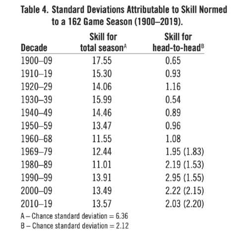
If the head-to-head factor plays no role in determining a team’s season record against each of the other teams, then we should expect that deviations of season records against specific teams from overall performance of a team should be a matter of chance. That is, when corrected for overall performance, teams would be expected to do equally well against each other on the average. Returning to the 1954 White Sox example, the number of victories corrected to reflect the head-to-head factor for each White Sox opponent produced an average of 11 games. The result reflects no advantage or disadvantage for one team against another on the average. It is possible to demonstrate that in general the expected value of number of season’s victories for one team against another is one half the games they play against each other⁷. For example, in a 162-game season two teams within a division generally play 18 games against each other with each team expected to win 9 games if no head-to-head factor is involved and there is no overall difference between the two teams. Thus, it is appropriate to use p =.50 to calculate variance attributable to luck in testing for significance of the head-to-head factor.

We can see that the skill standard deviation for total season wins per decades ranged from 11.01 for the 1980s to 17.55 for 1900–09. The corresponding ratio of skill to luck ranged from 1.73 to 2.76. Although there may have been a small drop-off in amount of performance attributable to skill post-1968, the skill factor still dominates, with a large part of perceived drop attributable to introduction of the divisional structure. The skill factor for head-to- head performance averaged 1.46 over decades. The values for the divisional decades may over correct for season length, and skill standard deviations without the correction are shown in parentheses. These values are somewhat lower than the corrected values. The analysis suggests that for a given team the unique matchup factor may account for between 1 and 1.5 games on the average in a given season’s series. This may prove significant when considering a team’s matchups against all the other teams.

However, it is necessary to consider the net effect over a season. For example, the White Sox in 1954 fared poorly against the Yankees, winning only seven games, but they compensated by beating the Red Sox 17 times. Overall season records conceal much of the dynamics of a season. A team’s season win record gives a smoothed-over description of a season’s performance. It is true that the net sum of variations in head-to-head victories from a team’s average is zero. However, the comparison of a team’s head-to-head profile to the performance of its opponents against each other presents a complex picture of a season. Unlike total season record, the head-to-head factor is only a little less than half of the luck factor of 2.12 standard deviations.

Measures of the effects of performance factors become meaningful only if they are reliably greater than would be expected by luck or random variation. Pearson’s Chi Square distribution provides a test of significance that allows us to determine the probability that the head-to-head factor is nothing more than the product of luck or random variation. A conservative statistical test was derived to determine this probability.⁸ Results for the head-to-head factor are shown in Table 5. All the results are significant at the .01 level. This means that it is very unlikely that the head-to-head factor reflects nothing more than luck. It is apparent that the head-to-head factor contributes a significant amount to performance differences. Corresponding chi square tests were done to test whether total season differences between teams are a matter of chance. For the total seasons’ records all results for decades through the 1970s were significant at the .01 level, the 1990s and 2010s were significant at the .05 level, and the 1980s and 2000s were nonsignificant.

 

 

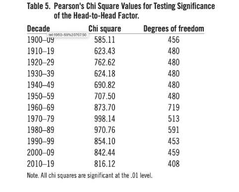
Next, I examined the relationship between overall season performance for teams and head-to-head performance. The analysis of variance enables us to see if the variance of season victory totals is significantly greater than that for head-to-head performance. This appears obvious, and the analysis of variance confirms it. The 387 analyses of variance found that variance for total season victories was significantly higher than that for head-to-head variance at at least the .05 level in 217 of the cases. Random differences between the two factors would predict significance for between 19 and 20 of such cases.

PREDICTING HEAD-TO-HEAD PERFORMANCE

What is the importance of the small variation in performance attributable to the head-to-head factor? Each game is, after all, a head-to-head contest and the outcome should at least in part depend upon the specific pattern of relative strengths and weaknesses of the two teams, in addition to the overall abilities of the teams in competition with all other teams in the league. I return to the 1954 White Sox example and their record against each of the seven other teams in the league. The White Sox only won seven of their 22 games against the Yankees. The deficit, corrected for overall difference between teams of 6.26 games, may have something to do with the unique matchup between the teams in addition to the difference between the teams in overall ability. Except for their head-to-head performance, the teams were nearly equal. Of course, both finished behind the Cleveland Indians, who won 111 games (and proceeded to be swept by the Giants in the World Series, perhaps more evidence for a specific head-to-head factor?)

The problem of explaining the 6.26 game corrected deficit on the White Sox part may be of interest to those who wish to predict how teams will fare against each other apart from their overall competitive records. A natural way to approach the problem is to examine how differences between the teams in important performance variables predict differences between the teams in the unique head-to-head performance factor. An extensive exploration is beyond the scope of this article, but I made an initial try using four seasons that indicated a strong effect of the head-to-head factor with two prime performance measures which seemed to be good candidates: AERA, park adjusted earned run average, and AOPS, a park adjusted measure of on base average and slugging. These statistics I used were from the 2005 Baseball Encyclopedia.⁹

Pete Palmer did extensive work demonstrating the effectiveness of OPS as a predictor of wins and why it works.¹⁰ ERA would seem to be an appropriate complement to that. In our White Sox example, the difference between the White Sox and Yankees in these two measures would be used to predict the White Sox disadvantage against the Yankees, 6.26 games. The difference in 1954 between the two teams in AERA was 122 – 105 = 17 favoring the White Sox; however the difference in AOPS favored the Yankees, 103 – 118 = –15. The Yankees that year were first in AOPS, a power-laden team that out-homered the White Sox 133 to 94. The White Sox defense, on the other hand, had an advantage. In this matchup the offensive factor seemed to outweigh the defense. It is necessary to see how these variables relate to each other and to the head-to-head factor.

I used season data for the 1905, 1909, and 1962 National League seasons and the 1954 American League season to test the predictive value of the two above performance measures for the head-to-head factor. The selected seasons seemed promising because the contribution of the head-to-head factor was strong for these seasons. Of course, further research would be necessary if results generalize. Stanley Rothman used runs scored minus run allowed as a predictor in a linear regression analysis predicting overall winning percentage.¹¹ His analysis was able to account for nearly 95% of variation in winning percentage. However, the predictor variable includes chance variation as well as variation attributable to skilled performance such as AOPS and AERA.

Multiple regression was used to generate a prediction equation of the form

a + b. (AOPS_{White Sox} − AOPS_Yankees) + c.(AERA_{White Sox} − AERA_Yankees)

using our White Sox-Yankees example for predicting the head-to-head effect in this case. Value predicted would be compared to the observed value of −6.26 in this case. The equation for a season would be arrived at by determining the values of the weights in the equation that best fit the set of head-to-head performance values for all pairs of competing teams. There were 28 pairs of teams in 1905, 1909, and 1954; and 45 such pairs in 1962. The prediction equations for each season contain weights that produced the highest multiple correlation between those equations and the head-to-head performance measures.

 

 

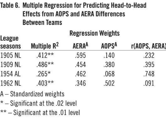
Table 6 shows the multiple correlation squared, weights for the two predictors, and correlation between the two predictors for each of the four seasons. Multiple R² was used, because it measures the proportion of total variance attributable to the two predictors. The correlations between the two predictors, r(AOPS, AERA), are shown, but the predictive weights indicate the contribution of each predictor apart from that of the other predictor. Although the number of team pairs in a season was not large, the multiple correlations between prediction equations and head-to-head measures were highly significant for all of the four seasons. Multiple correlations range from .515 to .697, where 1.000 is the maximum possible value. Standardized weights are shown, which makes the values comparable in terms of units of the variable measured. It is noteworthy that the AERA variable outweighed the AOPS variable in three of the four cases which highlights the importance of pitching in head-to-head matchups.

In exploring the variables that may correlate with the head-to-head factor it is well to be aware that the pattern of measures of this factor for teams at the top or bottom range of the standings differ from the pattern for teams near the middle. Teams near the top have a smaller chance of showing a positive head-to-head value over a given team than do teams lower in the standings. By the same token, losing teams have a better chance of showing a head-to-head advantage than do teams above them. The ceiling or floor in season performance makes this intuitive.

To illustrate for a winning team, consider the 1954 White Sox example again. The White Sox were 15 and 7 against the Orioles, demonstrating dominance. However, their score of 9.67 victories adjusted for relative performance of the two teams against the rest of the league placed them 1.33 games below the expected 11 game average against the league given no head-to-head effect. This, of course, results from the fact that the overall performance of the White Sox against teams in the rest of the league was on the average 5.33 games better than that of the Orioles. Thus, it appears that the White Sox underperformed against the Orioles.

As a counter example substitute a middle of the pack team with a 77 and 77 record for the White Sox which produces an average of 11 victories against each team in the rest of the league. This hypothetical team would have won half a game more on average against each of the rest of teams than did the Senators. If the hypothetical team beats the Senators 15 times, it has a four game advantage over its average. Subtracting the half game from this value produces a healthy 3.5 game head-to-head effect. Analogous comparisons to those above for losing teams would tend to result in apparent over performance. The above comparisons should be considered in evaluating head-to-head competition.

The results give support to the idea that unique factors associated with competition between certain teams can be assessed in understanding the dynamics of a season. Certainly, if measures associated specifically with head-to-head competition reflect only random variation, we could not expect any variables to provide significant predictive ability. Having an edge over another team in performance variables in five-team divisions assumes great importance.

 

Acknowledgments

I would like to acknowledge Rodger Payne for his helpful comments as I prepared this article.

 

Notes

8. Pythagorean expectation, “Pythagorean theorem of baseball,” Baseball-Reference Bullpen, https://baseball-reference.com/bullpen/pythagorean
9. Clay Davenport and Keith Woolner, “Revisiting the Pythagorean Theorem,” Baseball Prospectus, June 30, 1999, http://www.baseballprospectus.com/article.php?articleid=342
10. “W% Estimators,” http://gosu02.tripod.com/id69.html
11. Pete Palmer, “Calculating Skill and Luck in Major League Baseball.” SABR Baseball Research Journal 46, no.1 (2017): 56-60.
12. John A. Richards, “Probabilities of Victory in Head-to-Head Team Matchups,” SABR Baseball Research Journal 43, no.2 (2014): 107-117.
13. In general, twice the variance is equivalent to the average of all the squared differences between each of the possible paired observations in the distribution of values. If the correlation between pairs of observations is negative, it can be shown that the variance is greater than would be the case if observations were independent. In the period before 1969 and in intra-divisional play each team plays every other team an equal number of times, and the total number of victories within a division is fixed. The expected correlation between pairs of teams is then negative. Thus, the variance of team victories can be expected to be greater for intra-divisional play than for extra-divisional play, where observations are independent of each other.
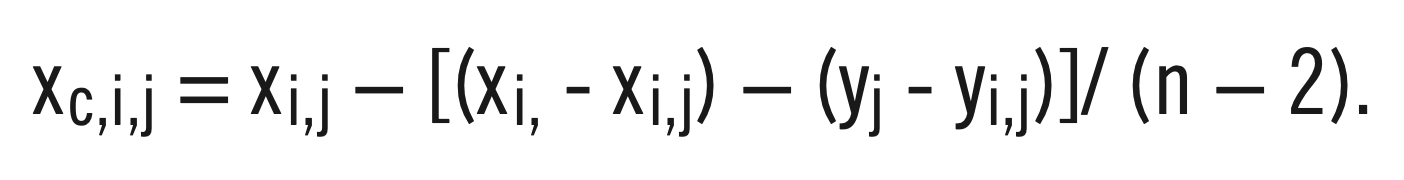
14. Consider corrected head-to-head values for a given team against another team in the same league or division, e.g., the White Sox against the Senators. Let x_i be total victories for team i, and let y_j be total victories for team j. Let x_i,j be the number of victories for team i against team j, and let y_i,j be the number of victories for team j against team i. Further let n be the total number of teams, e.g., eight in the 1954 American League. Then, the head-to-head correction for team i against team j is

    

    Next, consider average corrected head-to-head value for team i against the other n-1 teams. The average × (n-1) is,

    

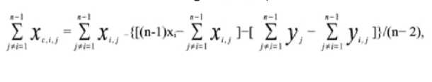
    where the subscript j is used to designate teams other than team i. Let N equal the number of games two teams play against each other in a season, e.g. 22 games in the 154 season. Next consider the following:

    

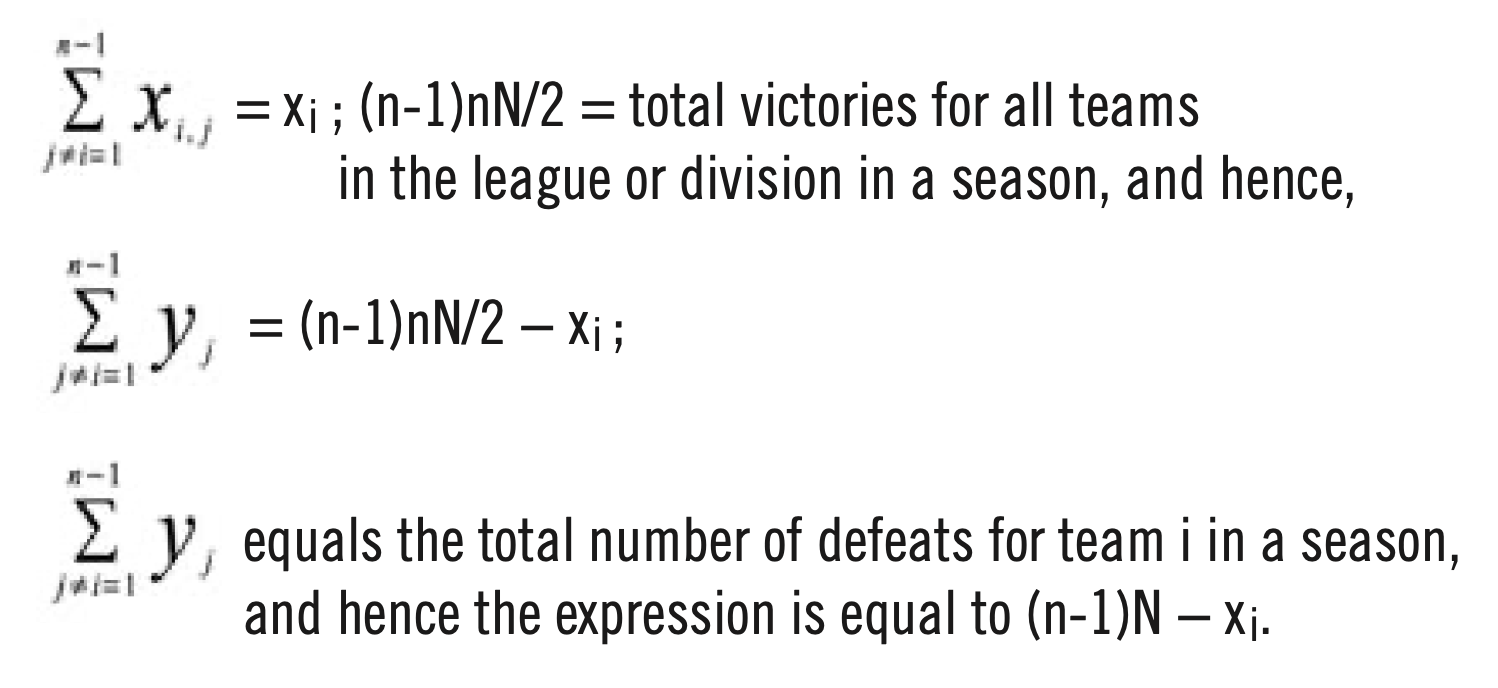
    Using these equivalences in the expression for the corrected head-to-head value and collecting terms gives us a value of (n-1) N/2. Thus, the average corrected head-to-head victories for a given team over teams in the rest of teams in the league is N/2.

15. The additive nature of the Chi Square distribution allows us to aggregate sums of squared differences as is in the White Sox example over all teams in a season and all seasons for a decade in order to make a comparison to the variance expected by pure luck. The significance test requires the assumption that observations are independent of each other. Because number of victories for one team in a series is inversely related to that for the other, there is a strong dependence between those values. If we hypothetically consider numbers for only one member of each pair, we can make a very conservative calculation by assuming a Chi Square value half as large as the one made for the complete set of values for each decade and use the Chi Square value needed for significance one half as large as that required for significance for all values. This adjustment plus the use of .50 in estimating chance variation likely produces an underestimation of the degree of statistical significance.
16. Pete Palmer and Gary Gillette, eds. The 2005 ESPN Baseball Encyclopedia (New York: Sterling Publishing Co., Inc., 2005).
17. Pete Palmer, “Why OPS Works,” SABR Baseball Research Journal 48, no.2 (2019): 43-47.
18. Stanley Rothman, “A New Formula to Predict a Team’s Winning Percentage,” SABR Baseball Research Journal 43, no.2 (2014): 97-105.