Tony Gwynn: Meeting Baseball’s Best Hitter

“I don’t like to compare myself to hitters of the past because people always start talking about eras — ‘Gwynn’s got to face four different pitchers in a game’ — all that stuff. Forget all that. It’s still the game of baseball. When I’m dead and gone, all that will be left is the numbers. They won’t remember how much heart a person had, or how consistent he was, they’ll just look at the numbers. And the numbers will tell you that I won eight batting titles; that I tied Honus Wagner for winning the most. The numbers will tell them that Wagner was a .345 lifetime hitter; and that I am a .340 lifetime hitter. So who was better? Honus Wagner. That’s how it will be judged.” — Tony Gwynn1

“Gwynn will look at tapes for hours. He has one tape of each team. Each tape has all his at-bats against that team in the season. He has a tape . . . featuring all his at-bats in the previous season.” — George F. Will2

“Relative to the right wall of human limitation, Tony Gwynn and Wee Willie Keeler must stand in the same place — just a few inches from theoretical perfections (the best that human muscles and bones can do). But average play has so crept up upon Gwynn that he lacks the space for taking advantage of suboptimality in others.”   — Stephen Jay Gould3

 

I met baseball’s best hitter! No, not Babe Ruth, who died in 1948. He is baseball’s best batter. No, not Ty Cobb, who died on my fourth birthday, in 1961. He is baseball’s best “unadjusted” hitter. Not Honus Wagner (who actually had a .328 lifetime batting average). Not Ted Williams. Not even Wee Willie Keeler! To a sabermetrician like me, adjustments are important — nay, critical — to evaluating player performance. The moniker “baseball’s best hitter” properly belongs to Tony Gwynn.

First, I should explain that the term “best hitter” is a vague one. I define it to be “best at getting hits.” The classic metric for this is batting average. Some baseball pundits prefer to say that batting average measures ability as a “pure hitter” rather than as a “hitter.” OK, fine. Call Gwynn “baseball’s best pure hitter.” Why should we even care about this title, though? Aren’t sabermetricians all about wins, wins, wins, which essentially comes from runs, runs, runs — so concepts like WAR (wins above replacement), OPS (on-base-plus-slugging), or linear weights become the metrics of choice? Well, this sabermetrician cares about more than wins. There is an art to hitting — baseball swings can be beautiful. Just watch a regular-season game. A single typically gets much more applause than a walk. In Internet terms, it gets more “likes.” Winning shouldn’t be everything, otherwise a late-season game between two non-contenders should just be canceled.

Oh, I define “best batter” (or perhaps “best all-around batter”) as the player with the best ability to produce runs (thus wins) in a given plate appearance, while “best player” is the best all-around player, which includes baserunning, fielding, and pitching abilities. Yes, Babe Ruth wins both of these awards.

Baseball-Reference.com shows Gwynn tied for 18th with Jesse Burkett and Nap Lajoie with a .3382 lifetime batting average in 18 seasons, all with the San Diego Padres.4 Meanwhile, Cobb steals the top spot with a .3662 mark. In my 1999 book, Baseball’s All-Time Best Hitters, I recommended that four adjustments be made to determine who really deserves to be called the “best hitter”: for late-career declines; league average; player talent pool; and ballpark.5 The second and fourth adjustments are now a standard part of sabermetric adjustment, although there isn’t consensus on how to most properly do so. The talent pool is a much more difficult adjustment to make, but the concern certainly pops up, especially when comparing players before and after integration in 1947. Some analysts identify a subset of years for a player as “prime years,” a version of the first adjustment. I won’t talk further of alternative adjustment methods, but simply apply what I think is the best analytic approach and report the results.

My adjustment for late-career declines uses only the first 8,000 at-bats of a player’s career. That led me to fly from North Carolina in late July 1997 to San Diego to see Tony Gwynn’s 8,000th at-bat. That week, Gwynn was on the cover of both Sports Illustrated and The Sporting News, as he was batting close to .400. SI had the provocative title “The Best Hitter Since Ted Williams,” who intriguingly was a San Diego native and the second-“best hitter” behind Cobb, using a league average-type adjustment.6 Notably, SI adopted the same definition as mine for “best hitter” and awarded Gwynn the sixth spot, using an obviously imperfect adjustment of the league average. It had two key imperfections: 1) the adjusting season average combined data from both leagues, though AL pitchers have rarely batted since 1973, a transition that resulted in a seven-point jump in the league batting average — thereby hurting Gwynn by 3.5 points; and 2) the composite league average wasn’t weighted by the player’s at-bats for each of the seasons. Had SI done that, Gwynn would have slipped past Williams into second, also getting past Hornsby, Lajoie, and Keeler. I wanted to meet Gwynn and tell him that he was the best hitter in spite of Williams.

In Best Hitters’ adjusted world, Gwynn edged Cobb by a razor-thin margin of nine adjusted hits, a gap of .0011 batting-average points. The talent pool adjustment was based upon the standard deviation of “regular players,” defined later. Having made improvements on this estimate, my second book, Baseball’s All-Time Best Sluggers (called Best Sluggers hereafter), concluded that Gwynn won by 22 adjusted hits.7 The third-place hitter, Rod Carew, was six to eight points of average back in the books, effectively making it a two-man race. Today, we can improve the comparison of Gwynn vs. Cobb, as the ballpark effects are better known. The ideal data to have are the home and road park batting data for all teams. While those were available for Gwynn when the books were written, only recently has Retrosheet had the park data for all but one of Cobb’s seasons (1905–28).

Adjustment 1: Late-Career Declines

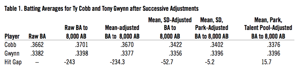
Perhaps the most arbitrary adjustment is for late-career declines. I thought some milestone number was needed that was close to a full career for most players but would allow us to trim off some late years when most players’ averages drop off. 8,000 AB was my choice then, and I still think it is a good one. In my view, identification of the “best hitter” shouldn’t be affected by the player’s wisdom in choosing his retirement date. Cobb gains about four points and Gwynn gains two by restricting batting average to 8,000 AB.8 Gwynn became the 104th player to reach 8,000 ABs. Up through that time, only six players had higher lifetime batting averages than they did at 8,000 AB, with only one player being among the top 100 adjusted best hitters — Roberto Clemente. For such rare exceptions, I adopted the rule of using the superior average when it occurred, either at a higher milestone number of ABs or the full career. Neither Cobb nor Gwynn was an exception. At this first adjustment stage, Cobb is 243 hits ahead of Gwynn.

Adjustment 2: League Average

 This adjustment is extremely well-ingrained among sabermetricians. The adjustment calls for dividing the player’s batting average by the league BA, either to obtain a “relative batting average,” or to be reconstituted using a benchmark BA. I have scaled it to a .270 batting average, the typical BA for “regular” players in the NL in 1969–92, when the average league average was .255. “Regular players” are the players with the most plate appearances in the season, using a cutoff such that about 75 percent of the plate appearances are included. Thus, pitchers and most pinch hitters would be excluded. Note that some early sabermetricians mistakenly believed that the player’s numbers should be removed from the league BA. All players are part of the league average, and in equally talented leagues with more teams, one should expect proportionally more great players; thus, it would be a bias to simply remove only the player of interest. This adjustment, while a quite powerful one, especially in adjusting the elevated average seen in the early live-ball era, say 1920–36, drops both Cobb’s and Gwynn’s averages only by a couple of points.

The table below shows the results after the four successive adjustments, the next two of which will now be described.

 

Table 1. Batting Averages for Ty Cobb and Tony Gwynn after Successive Adjustments

(Click image to enlarge)

 

Adjustment 3: Talent Pool

This adjustment, from a statistician’s perspective, is simply a two-moment adjustment. Having obtained the batting average distribution for regular players (on a square-root scale, as this is more closely normally distributed), we are scaling the batting performance by the first two moments — the mean and the standard deviation. In my two books, I called this a “talent pool” adjustment, which it is. It is a powerful adjustment, especially for players in a newly established league. It is somewhat imperfect, however, as will be discussed further later. The concept is that when the standard deviation is larger, it shows a greater spread in the distribution of averages — because weaker players are getting significant ABs. In two well-known publications, Stephen Jay Gould highlighted the importance of this heterogeneity (spread captured by the standard deviation) as illustrative of weakness in an evolving system, such as baseball was in its early days.9 Cobb played in a newly formed American League, joining the league in its fifth major-league season. Consequently, his average drops 25 points, and his hit lead narrows dramatically from 234 to 53.

Adjustment 4: Park Effect

This is another well-ingrained adjustment among sabermetricians. The principal adjustment that is used is one based on run-scoring, contrasting runs scored by both teams in a given park compared with those obtained when the given park’s home team plays on the road. It is better to adjust specifically for the event that one wants to adjust to rather than using the runs-based adjustment. My books described an adjustment, using home and road data for hits. Retrosheet now has park data back to 1906, so a more accurate park effect based on the exact data became possible for Cobb. The books had used an approximation method for Cobb’s parks; overall, the approximation method had a Pearson correlation of 0.75 with the exact data when both were available.10 The new results change the story rather dramatically. Navin Field, which Cobb played in from 1912 until 1926, which Best Sluggers had rated as giving Cobb an extra seven batting points per season, is actually a neutral park for hits. With the new, improved park data, Cobb wins by 5.2 hits rather than loses by 22!

Does that mean that I now believe Cobb is the best hitter? Well . . . according to the four-adjustment method laid out in my books, yes. However, the talent pool adjustment, which was applied as Adjustment 3, was also known to be imperfect. As noted in Best Sluggers: “The primary assumption that a 90th percentile player in say, 1901, would be a 90th percentile player today is not likely to be true for each offensive event.”11 It also assumes that an average player in 1901 is like an average player today as well — essentially by calculating the batting average distance to the average player scaled by the standard deviation. While the excess distance attained from the early years was shrunk to not excessively favor them, the average player from a newly formed league was not simultaneously determined to be worse. In summary, the talent pool adjustment used in step 3 substantially reduced, but did not eliminate, the advantage of playing in an inferior league.

Best Sluggers described nine steps in the development of an ideal adjustment system, with development to that time being to step 5 — use of the batting average as a measure, with the four adjustments just described.12 Step 6 was an “improved estimation of park effects,” which was just reported above. Step 7 is a better assessment of the “changing ability of an ‘average player’ over history.” Below, I present a partial movement forward on this step. Steps 8 and 9 are still beyond our current analysis.

A New and Improved Talent Pool Adjustment

The standard deviation (SD) adjustment that comprised the third adjustment essentially equilibrates the players from all eras of play based on their percentile rankings in their seasons. While it did curtail the breakaway numbers of the superior players from weak talent pool seasons, it didn’t further penalize them by considering the average player to be inferior. Let’s look at the SDs for the first 25 AL major league seasons in five-year averages:

 

Table 2. Standard Deviations (SDs) of “Regular” Players in the American League in 5-Year Intervals

Years	SD
1901–05	.0322
1906–10	.0326
1911–15	.0362
1916–20	.0343
1921–25	.0300

 

It is highest for 1911–15. Does this mean that the AL got worse after the first decade, before subsequently improving? Actually, the increased SD coupled with our knowledge of the league provides evidence of an improving league, one that became more heterogeneous as more mediocre hitters were being replaced by better hitters. Who were these hitters? They included: Ty Cobb (first year as a regular player: 1906), Eddie Collins (1908), Frank Baker (1909), Tris Speaker (1909), and Shoeless Joe Jackson (1911). Notably, Cobb, Jackson, and Speaker all appear in Best Sluggers as adjusted top 10 “hitters.” The improved adjustment is to apply the elevated average SD of the three highest years, 0.0363 (1911–13) to 1901–10 as well, as they represented lower talent pool seasons. The earlier seasons were likely worse; however, I don’t yet know how to demonstrate that. I am asserting via revised talent pool adjustment that they weren’t better. Two additional changes should be made as well: 1) when calculating a player’s Z-score, rather than subtracting off the transformed mean from the season one should subtract off the standardized average (.5191 on the square-rooted scale), and 2) one should divide by the standardized SD, .0263, rather than the SD from the season whenever the player hits below average (this prevents elevation of subpar performances in a poorer talent pool season).

Conclusion

The new talent pool approach reduces Cobb’s hit total by 20.8, from the seasons 1905–10. Thus, Cobb, with a .3376 average, finishes 15.7 hits behind Gwynn and his .3396 average. Further improvement of talent pool adjustment is needed; however, it would only further reduce Cobb’s hits relative to Gwynn. As Cobb has already dropped below Gwynn in his adjusted hit total, we may conclude, albeit by the slimmest of margins (about a hit per season), that Tony Gwynn is the best hitter of all time!13

Interestingly, Best Sluggers concluded that Tony Gwynn was also the best at not striking out. George Will certainly made a good choice of Tony Gwynn as the primary focus of the chapter “The Batter” in Men at Work.14

Meeting Tony Gwynn

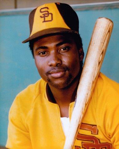
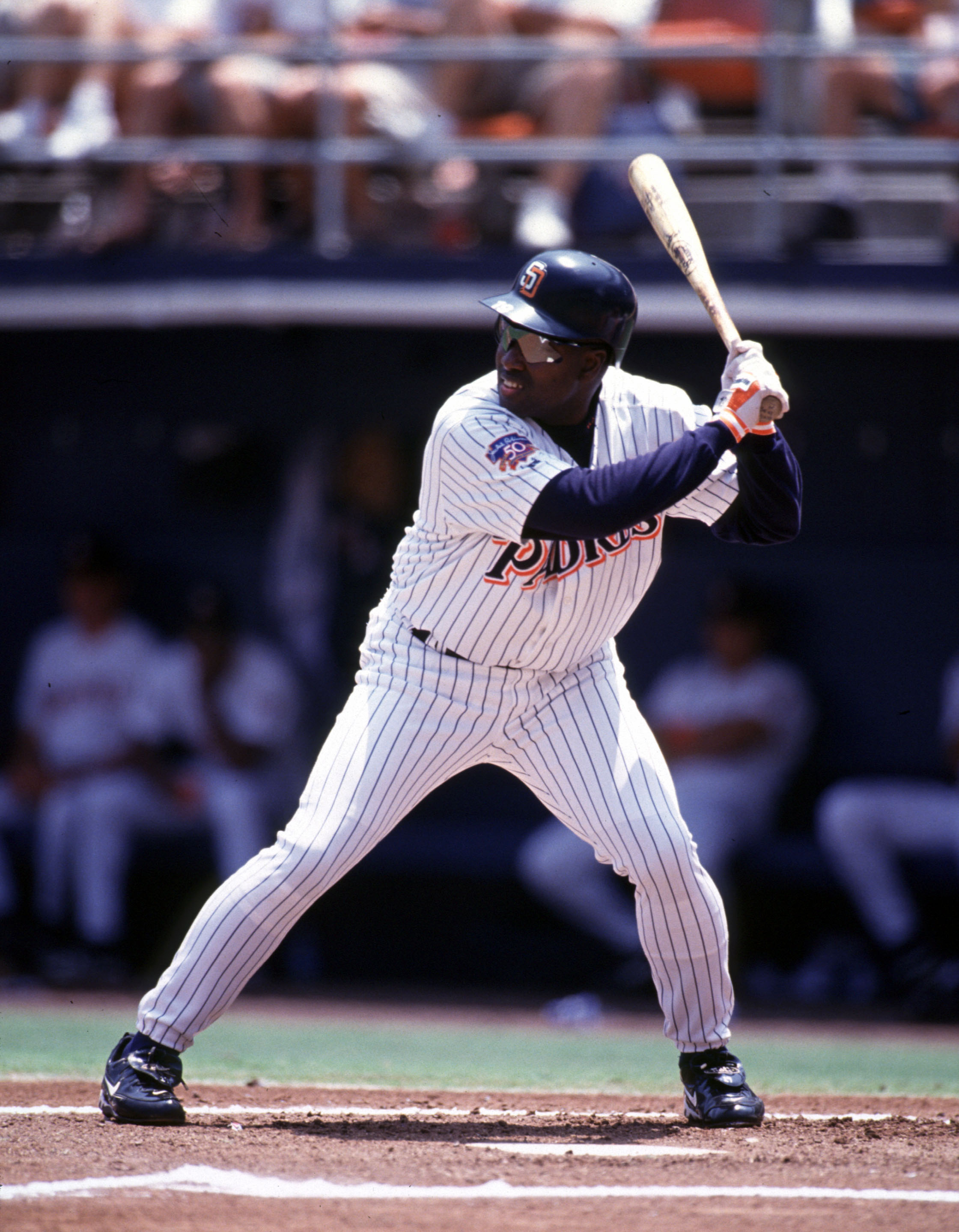
I met Tony Gwynn, baseball’s best hitter, on July 28, 1997, a couple of hours before he singled in his 8,000th career at-bat. He was very gracious. I gave him a copy of Gould’s “Entropic Homogeneity” article and briefly explained why the current SI article by Tom Verducci had not adjusted the batting averages well enough (data analysis came from the Elias Sports Bureau).15 Gwynn, in turn, gave me a bat, one that he said “had hits on it” — and also hand-drawn racing stripes, which I think he must have done himself. What other player batting .391 in late July would give away one of his game bats? The day Gwynn died, I was called by Jay Caspian Kang of the New Yorker. I told Kang that the only way for Gwynn to be shown to be baseball’s best hitter was through the adjusted batting average by a statistician, and that “I was his statistician.”16 I am honored that my name has been linked to Tony Gwynn’s, who is baseball’s best hitter.

Mr. Padre — we DO remember your heart and we don’t just look at the raw numbers.

MICHAEL J. SCHELL has been a SABR member since 1998, is a Senior Member in the Biostatistics and Bioinformatics Department at the Moffitt Cancer Center in Tampa, Florida. His two books, “Baseball’s All-Time Best Hitters” (1999) and “Baseball’s All-Time Best Sluggers” (2005), adjust player statistical data for era of play, talent pool, ballpark, and career longevity. His most provocative conclusion is that Tony Gwynn is the “best hitter” in baseball history.

 

Notes

1  Tony Gwynn, with Roger Vaughan, The Art of Hitting (New York: GT Publishing, 1998), dedication page.

2  George F. Will, Men At Work, (New York: Macmillan, 1990), 221.

3  Stephen Jay Gould, Full House: The Spread of Excellence From Plato to Darwin (New York: Three Rivers Press, 1996), 114.

4  “Career Leaders & Records for Batting Average,” Baseball-Reference, https://www.baseball-reference.com/leaders/batting_avg_career.shtml

5  Michael J. Schell, Baseball’s All-Time Best Hitters (Princeton: Princeton University Press, 1999).

6  Tom Verducci, “The Best Hitter Since Ted Williams,” Sports Illustrated, July 27, 1997.

7  Schell, Baseball’s All-Time Best Sluggers (Princeton: Princeton University Press, 2015).

8  Retrosheet data allowed me to get the hits totals exactly.

9  Gould, Full House; Gould, “Entropic Homogeneity Isn’t Why No One Hits .400 Any More,” Discover, August 1986.

10  Schell, Baseball’s All-Time Best Hitters, 118.

11  Schell, Baseball’s All-Time Best Sluggers, 214.

12  Schell, 212.

13  If one doesn’t apply the late-career decline adjustment, Gwynn easily wins: .3374 to .3299.

14  Will, Men At Work.

15  Verducci, “The Best Hitter Since Ted Williams”; Gould, Full House; Gould, “Entropic Homogeneity.”

16  Jay Caspian Kang, “Tony Gwynn: An Appreciation,” New Yorker, June 16, 2014. https://www.newyorker.com/sports/sporting-scene/tony-gwynn-an-appreciation