A New Formula to Predict a Team’s Winning Percentage
This article was written by Stanley Rothman
This article was published in Fall 2014 Baseball Research Journal
Bill James introduced a formula for estimating a team’s expected winning percentage in the major leagues based on the number of runs they scored and allowed. Empirically, this formula correlates fairly well with a team’s observed (actual) winning percentage, W%. Here is the so-called “Pythagorean” formula for baseball:
EXP(W%) = (RS)2 / [(RS)2 + (RA)2]
EXP(W%) is the expected winning percentage generated by the formula, RS is runs scored by a team, and RA is runs allowed by a team. It is understood that (RS)2 / [(RS)2 + (RA)2] is actually a ratio and needs to be multiplied by 100 to be a percentage.
James’s choice of the exponent 2 seems to provide a good estimate. From year to year, the exponent actually varies from 1.75 to 2.05. James’s rationale is that the number of runs a team scores compared to the number of runs allowed is a better indication of a team’s future performance than their win-loss record at a given time (assuming the team is far enough into the season for significance). This reasoning is the antithesis of the famous Bill Parcells quotation: “You are what your win-loss record says you are.” Let’s say a team is 45-37 at midseason, but based on James’s formula their EXP(W%) is at or below 0.500. The formula predicts that as the season moves along, their won-loss record will move in the losing direction.
Why not just use the quantity (RS – RA) to calculate EXP(W%)? The new formula we introduce here is called the Linear Formula for Baseball, and takes the form of the following linear equation.
EXP(W%) = m*(RS – RA) + b.
The tool used to find the coefficients “m” and “b” is simple linear regression. For each year from 1998 through 2012 we demonstrate that
m = Σ[RS-RA]W% / Σ(RS-RA)2 and b = 0.50.1
Given that we find the value for “m” will vary from year to year while the value “b” will remain fixed at 0.50, can one constant be found for the slope “m” that can be used for each year? This constant would work like the exponent “2” works for each year in James’s formula. The constant turns out to be m = 0.000683.
A final comparison is done between the Pythagorean Formula and our new Linear Formula for 2013.
The same methods used in this paper for Major League Baseball will be used to provide linear formulas for the NFL and the NBA. For the NFL, m = 0.001538, b = 0.50 and for the NBA, m = 0.000351, b = 0.50. The only change is that for the NBA and NFL the difference (RS – RA) will be interpreted as the difference (PS – PA) (points scored – points allowed). The actual derivations will be provided in a section near the end of this paper.
A Simple Linear Regression Model To Predict An MLB Team’s Winning Percentage Using (RS – RA).
Given n ordered pairs (x,y), the standard simple linear regression equation is:
y′ = m*x + b
m = [nΣxy – (Σx)(Σy)] / [nΣx2 – (Σx)2]
b = [(Σy)(Σx2) – (Σx)(Σxy)] / [nΣx2 – (Σx)2]
Equation 1
In our model for simple linear regression, n will be the 30 teams in MLB. For each team, x will be the difference between their runs scored and runs allowed (x = RS – RA), y will be their actual observed winning percent (W%) and y′ is the team’s expected winning percentage EXP(W%) based on (RS – RA).
For each year 1998-2012,
Let W = total wins for an MLB team
Let T = 162 games played by an MLB team
It is easy to see:
(1) Σx = Σ(RS – RA) = 0
(2) Σy = ΣW% = (1/T)*ΣW = (1/T)*(n/2)T = n/2 = 15
(3) Σxy = Σx*W% = Σ(RS – RA)W%
Replacing Σy with (n/2), Σx with 0, and Σxy with Σ(RS – RA)W% in Equation 1, the coefficients “m” and “b” become:
(4) b = [(n/2)Σ(RS – RA)2 – 0] / [nΣ(RS – RA)2 – 0]
b = 0.50(5) m = [nΣ(RS – RA)W% – 0] / [nΣ(RS – RA)2 – 0]
m = Σ(RS – RA)W% / Σ(RS – RA)2
Equation 1 turns into Equation 2 for each team for the years 1998-2012.
y′ = EXP(W%) = [Σ(RS – RA)W% / Σ(RS – RA)2]*(RS – RA) + 0.50
Equation 2
The above derivation is based on the assumption that each team played their scheduled T = 162 games. In some years a few teams either play one game more or less than the 162 games. This can happen when a rained out game is not made up because the game has no effect on the standings or when an additional game is forced by a tie for a playoff spot, as happened in 2009 and 2013. In 2009, the Σy in (2) above was 15.0020 and in 2013, Σy in (2) above was 15.0062. In 2009, (4) above will have b = 0.5001 and in 2013, (4) above will have b = 0.5002. Since the calculation of “m” in (5) above is not affected by the Σy, replacing b = 0.50 by either b = 0.5002 or b = 0.5001 in Equation 2 above will change the expected winning percentage y′ in the 4th decimal place. Clearly, this has basically no effect on y′.
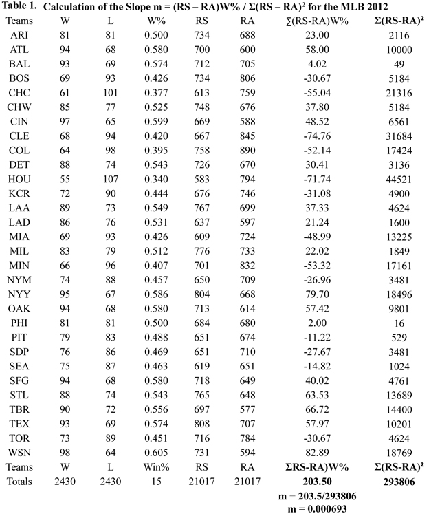
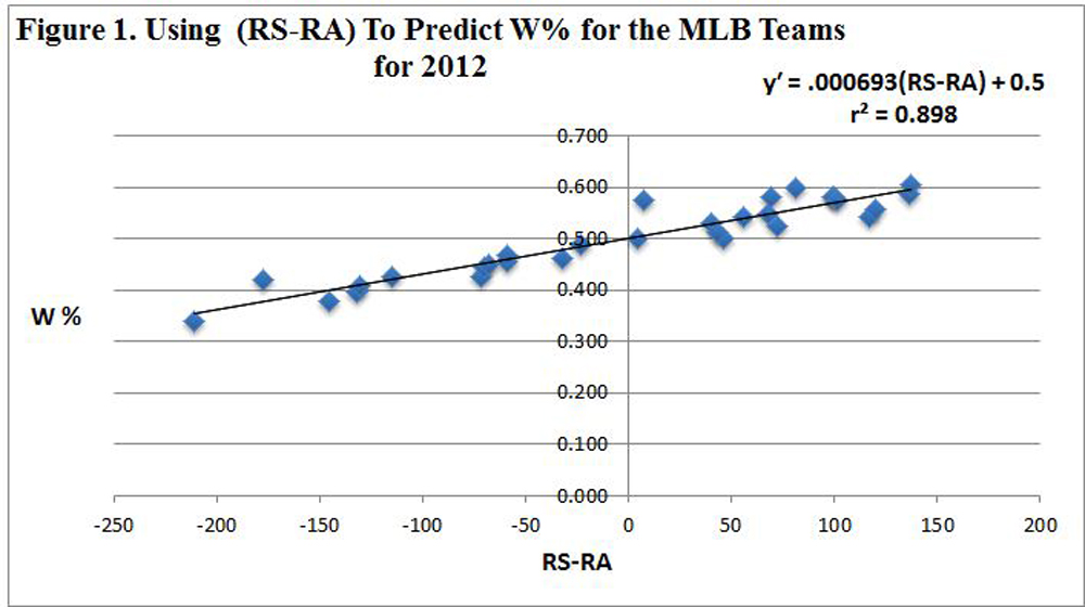
Table 1 (click link for image or see below) shows the calculation of the slope m = Σ(RS – RA)W% / Σ(RS – RA)2 = 203.50/293806 = 0.000693 for the MLB for 2012.
Figure 1 shows the scatter diagram, the regression line, the linear regression equation, and the coefficient of determination, r2, for MLB in 2012.
A Simple Linear Regression Model To Predict A League’s Yearly Σ(RS – RA)2 Using Σ(RS – RA)W%
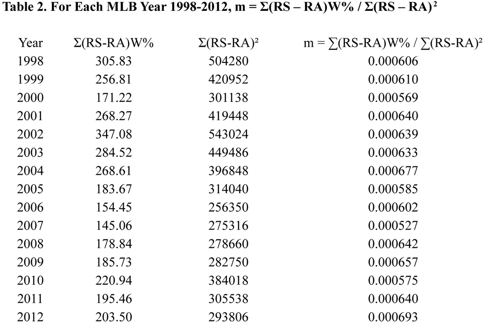
For each year 1998-2012, let x = Σ(RS – RA)W%, y = Σ(RS – RA)2 , and y′ = EXP(Σ(RS – RA)2), the expected yearly Σ(RS – RA)2. Table 2 (click link for image or see below) shows the x and y values and the slope “m” for each of the years 1998–2012. The values of the slopes range from a low of 0.000527 to a high of 0.000693.
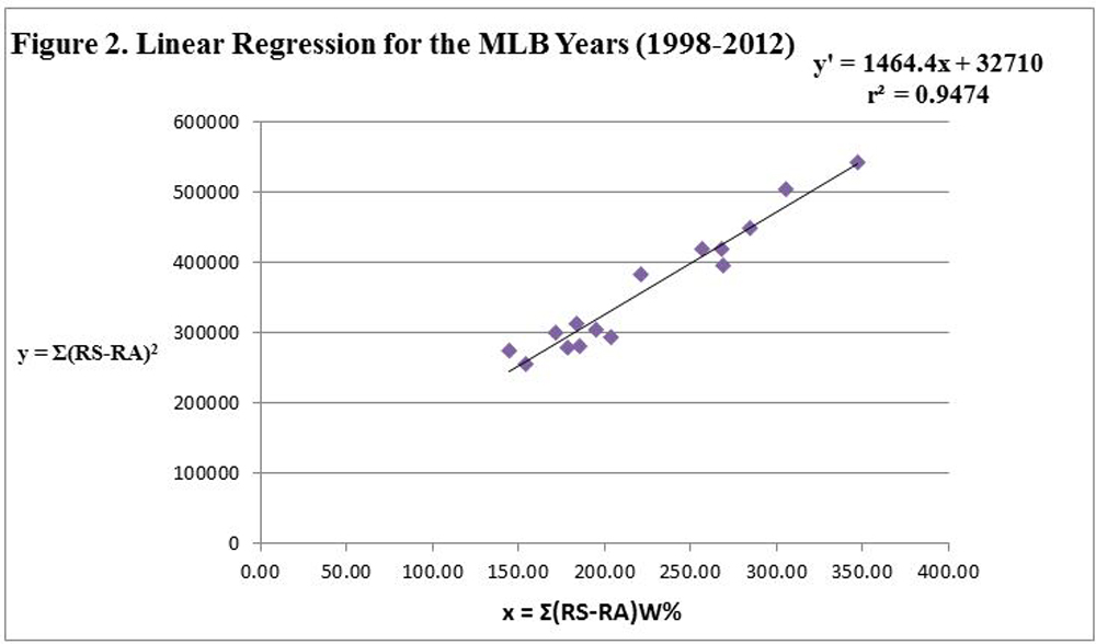
Figure 2 provides the linear regression equation, the graph of the regression line, and the coefficient of determination, r2, for the years 1998-2012. The linear regression equation using x = Σ(RS – RA)W% to predict y = Σ(RS – RA)2 and the corresponding coefficient, r2, is given as Equation 3 below.
y′ = EXP(Σ[RS – RA]2) = 1464.4Σ[RS – RA]W% + 32,710
r2 = 0.9474
Equation 3
Finding One Slope To Use As An Estimate For Each Year For MLB
Because of the strong positive correlation between x = Σ(RS – RA)W% and y = Σ(RS – RA)2 in Equation 3, we can replace Σ(RS – RA)2 in Equation 2 with 1464.4Σ(RS – RA)W% + 32,710 (from Equation 3) giving us Equation 4 below for the expected winning percentage for a team.
EXP(W%) = [Σ(RS – RA)W% / [1464.4Σ(RS – RA)W% + 32,710]]*(RS – RA) + 0.50
Equation 4
Since for each year 1464.4Σ(RS – RA)W% is greater than 212,418.5 (see Table 2) which is much greater than 32,710, we can replace 32,710 with 0 in Equation 4 yielding a final approximation for the expected winning percentage for any team for the years 1998-2012 in Equation 5 below.
EXP(W%) = [Σ(RS – RA)W% / 1464.4Σ(RS – RA)W%]*(RS – RA) + 0.50
= (1/1464.4)*(RS – RA) + 0.50
= 0.000683(RS – RA) + 0.50
Equation 5
An Application Of The Linear Formula For Baseball
For a team to increase its winning percentage for a year by one percentage point, a team would need to increase the difference (RS-RA) by approximately 14.64 runs (0.01/0.000683). If a team won 81 games last year (50 percent of its games) and we believe that if a team wins 90 games, (winning 55.56 percent), they have a good chance of making the playoffs, the yearly difference (RS-RA) should increase by 14.64*5.55 = 81.25 runs. A general manager could use this information to improve his team based on the previous year’s RS and RA.
Comparing Linear and Pythagorean Formulas
For this comparison we will look at the 2013 regular season and compare the Pythagorean formula [EXP(W%) = RS2 / (RS2 + RA2)] with my Linear Formula for Baseball [EXP(W%) = 0.000683(RS – RA) + 0.50].
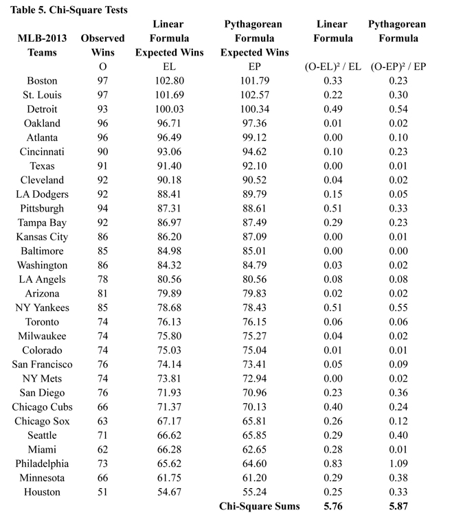
To test the hypothesis that each formula’s predicted expected win totals for a team is a reasonable estimate for the team’s actual win totals, we used the well-known Chi-Square Goodness-Of-Fit Test. Table 3 provides the expected win totals for each MLB team for 2013 using the Linear Formula.
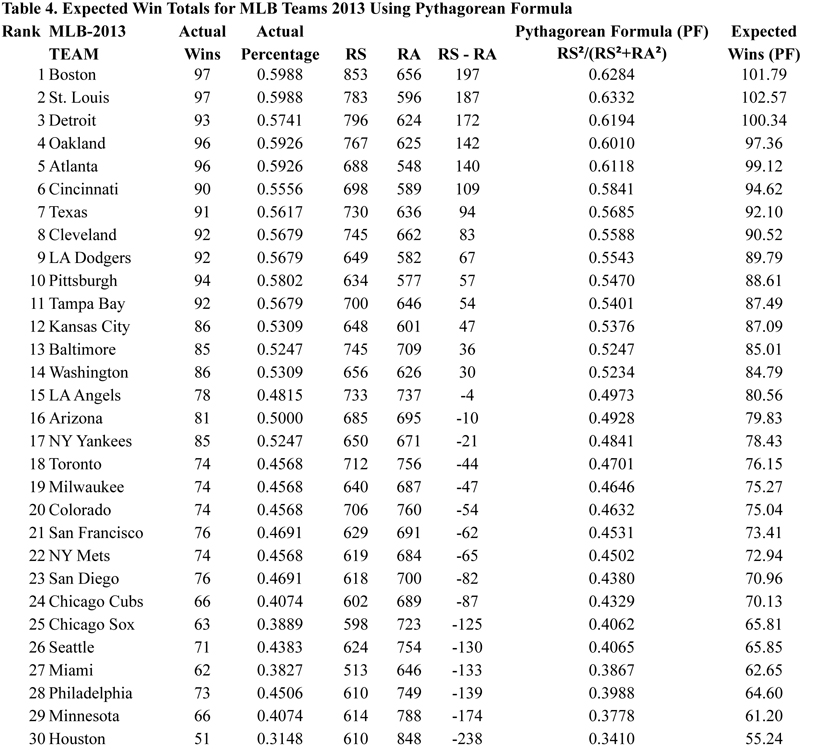
Table 4 (click link for image or see below)provides the expected win totals for each MLB team for 2013 using the Pythagorean Formula. The chi-square sums are 5.76 for the Linear Formula and 5.87 for the Pythagorean Formula (see Table 5 below). The p-values (the probabilities of these two small chi-square sums occurring strictly by chance if we believe the two formulas are accurate) are both greater than 0.90 (using 29 degrees of freedom). This indicates there is no reason to believe that both of these formulas cannot be used to predict a team’s expected winning percentage for the 2013 season.
Observe in Table 3 (click link for image or see below), using the Linear Formula, the top 11 expected winning percentages belong to the 10 teams that made the playoffs in 2013. The extra team was caused by a tie between Tampa Bay and Texas.
Extending The Linear Formula For Baseball To The NFL and NBA
We will now use the same techniques to develop Equations 2, 3, 4, and 5 for the National Football League and National Basketball Association. For these two leagues, x = (points scored (PS) – points allowed (PA)) and y = W%. Notice PS and PA replace RS and RA but have the same meaning.
Since (1), (2), (3), (4), and (5) below remain the same for the NFL and NBA, Equation 2 is the same for the NFL and NBA. The fact that T and n may be different for the three leagues had no effect on the final results for “m” and “b”.
(1) Σx = Σ(PS – PA) = 0
(2) Σy = ΣW% = (1/T)*ΣW = (1/T)*(n/2)T = n/2
(3) Σxy = Σ(x*W%) = Σ(PS – PA)W%
(4) b = [(n/2)Σ(PS – PA)2 – 0] / [nΣ(PS – PA)2 – 0]
b = 0.50(5) m = [nΣ(PS – PA)W% – 0] / [nΣ(PS – PA)2 – 0]
m = Σ(PS – PA)W% / Σ(PS – PA)2
Equation 2 is given below.
y′ = EXP(W%) = [Σ(PS – PA)W% / Σ(PS – PA)2]*(PS – PA) + 0.50
Unlike in MLB, Item (2) above is always true in the NBA and NFL.
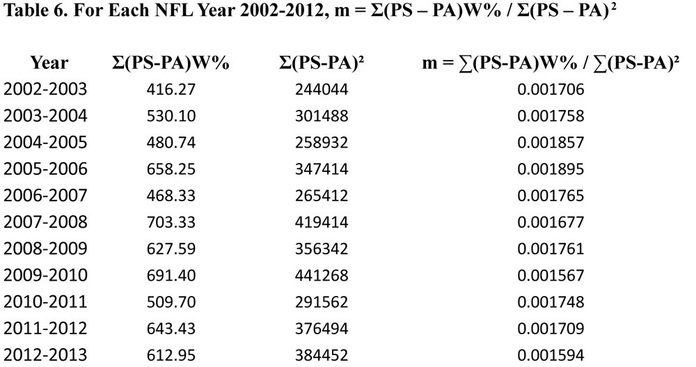
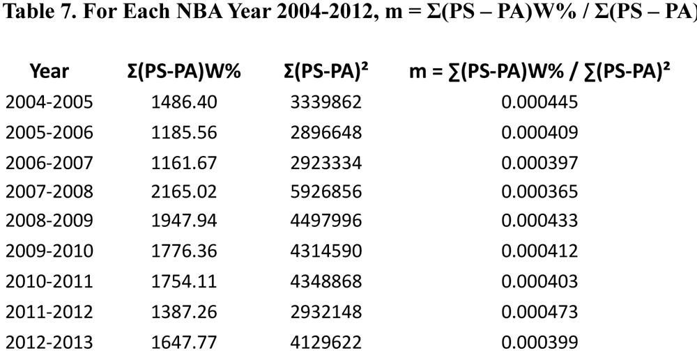
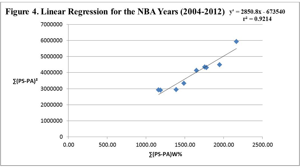
For each year 2002–12 for the NFL and for each year 2004–12 for the NBA, let x = Σ(PS – PA)W%, y = Σ(PS – PA)2 , and y′ = EXP(Σ(PS – PA)2), the expected yearly Σ(PS – PA)2 . Below is Equation 3 for the NFL and Equation 3 for the NBA (see Tables 6 and 7 along with Figures 3 and 4).
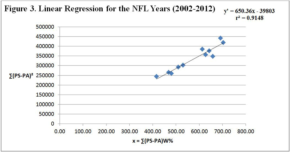
For the NFL, y′ = EXP(Σ(PS – PA)2) ′= 650.36Σ(PS – PA)W% – 39,803 (Equation 3)
and r2 = 0.9148.For the NBA, y′ = EXP(Σ(PS – PA)2) = 2850.8Σ(PS – PA)W% – 673,540 (Equation 3)
and r2 = 0.9214.
Because of the strong positive correlation between x = Σ(PS – PA)W% and y = Σ(PS – PA)2 in Equation 3 for both the NFL and NBA (see Figures 3 and 4), we can use 650.36Σ(PS – PA)W% – 39,803 (from Equation 3) to replace Σ(PS – PA)2 in Equation 2 for the NFL and 2850.8Σ(PS – PA)W% – 673,540 to replace Σ(PS – PA)2 in Equation 2 for the NBA yielding a new Equation 4 for the NFL and a new Equation 4 for the NBA.
For the NFL, EXP (W%) = [Σ(PS – PA)W% / [650.36Σ(PS – PA)W% – 39,803]]*(PS – PA) + 0.50. (Equation 4)
For the NBA, EXP (W%) = [Σ(PS – PA)W% / [2850.8Σ(PS – PA)W% – 673,540]]*(PS – PA) + 0.50. (Equation 4)
Since 650.36Σ(PS – PA)W% is greater than 270,722.1 for each year of the NFL (see Table 6) which is much greater than 39,803 and 2850.8Σ(PS – PA)W% is greater than 3,311,685 for each year in the NBA (see Table 7) which is much greater than 673,540, we can replace 39,803 with 0 in Equation 4 for the NFL and 673,540 with 0 in Equation 4 for the NBA yielding our final approximations for winning percentages in Equation 5 for the NFL and Equation 5 for the NBA below.
For the NFL, EXP (W%) = [Σ(PS – PA)W% / 650.36Σ(PS – PA)W%]*(PS – PA) + 0.50
= (1/650.36)*(PS – PA) + 0.50 = 0.001538(PS – PA) + 0.50. (Equation 5)For the NBA, EXP (W%) = [Σ(PS – PA)W% / 2850.8Σ(PS – PA)W%]*(PS – PA) + 0.50
= (1/2850.8)*(PS – PA) + 0.50 = 0.000351(PS – PA) + 0.50. (Equation 5)
The final versions are therefore:
The Linear Formula for NFL Football is EXP (W%) = 0.001538(PS – PA) + 0.50.
The Linear Formula for NBA Basketball is EXP (W%) = 0.000351(PS – PA) + 0.50.
Dividing 0.01 by 0.001538 tells us that each increase of 6.5 points for (PS – PA) will increase an NFL team’s winning percentage by an additional one percentage point. Dividing 0.01 by 0.000351 tells us that each increase of 28.5 points for (PS – PA) will increase an NBA team’s winning percentage by an additional one percentage point.
Conclusion
Using the Chi-Square Goodness-Of-Fit Test for both the Linear Formula and the Pythagorean Formula, we showed both were effective in predicting the actual win totals for the 2013 MLB season. We believe these two formulas will remain as effective in future years.
One advantage of the Linear Formula over the Pythagorean Formula is it is easier for a general manager to understand and use. A general manager can adjust either the runs scored or runs allowed—or both—when evaluating improvements to a team. Using the difference between the runs scored and runs allowed in the previous year as a starting point, a GM can plan to increase that difference to benefit his team. Of course, most teams (excluding the Yankees, Red Sox, and Dodgers) are constrained by budget. Upgrading the roster with players with underappreciated run-producing statistics but lower salary demands is one way to increase the RS component of (RS – RA) without overpaying for glitzier stats.
On the runs allowed side, a team might weigh the addition of one strong starting pitcher versus two lower-salary good starting pitchers to reduce the RA component. A second advantage of the Linear Formula is the same techniques used to develop the Linear Formula for Baseball applied to other sports leagues such as the NBA and NFL, and the same team-building advantages applied.
Two new research questions are born from these results. Why is there a strong positive correlation between ∑(RS – RA)2 and ∑W%(RS – RA) in MLB, the NFL, and the NBA? And how many games must be completed within a season for the Linear Formula to be an effective tool for predicting winning percentages in these leagues?
STANLEY ROTHMAN received his Ph.D. in Mathematics from the University of Wisconsin in 1970. In the fall of 1970 he joined the Quinnipiac University faculty as an Assistant Professor of Mathematics. He was promoted to full professor in 1982. He chaired the mathematics department at Quinnipiac from 1992 to 2010. In 2013, he began his 44th year at Quinnipiac. His book “Sandlot Stats: Learning Statistics with Baseball” was published in September 2012 by Johns Hopkins University Press. His book teaches an introductory statistics course using data from baseball. He has spoken at many universities including The West Point Military Academy and California State University at Los Angeles. He also has spoken at several math conventions, at high schools and at various community organizations. Some of his speaking topics include his own research on the probability of a player achieving various batting streaks, the probability of having another .400 hitter, and the role of minorities in baseball. His email address is stanley.rothman@quinnipiac.edu.
Additional points:
1. If RS – RA > 732 the linear formula for baseball, EXP(W%) = 0.000683(RS – RA) + 0.50, can yield an EXP(W%) > 100%. However, this is not a problem because for the years 1998–2012 the maximum value for (RS – RA) is 300.
2. If PS – PA > 325 the linear formula for football, 0.001538(PS – PA) + 0.50, can yield an EXP(W%) > 100%. However, this is not a problem because for the years 2002–12 the maximum value for (PS – PA) is 208.
3. If PS – PA > 1425 the linear formula for basketball, 0.000351(PS – PA) + 0.50, can yield an EXP(W%) > 100%. However, this is not a problem because for the years 2004–12 the maximum value for (PS – PA) is 691.
4. The scoring data needed for the discussion after Equation 2 and for Figures 3 and 4 can be found at the ESPN.com under the heading MLB and subheading Standings. Under the subtopic Standings you can retrieve the data (PS – PA), (RS – RA), and W%.
Sources
Wikipedia. http://en.wikipedia.org/wiki/Pythagorean_expectation. “Pythagorean Expectation.”
“The Pythagorean Theorem of Baseball.” http://www.baseball-reference.com/bullpen/Pythagorean_Theorem_of_Baseball.
Retrosheet. http://www.retrosheet.org.
Notes
1 The reason for starting with 1998 is this was the first year that there were 30 MLB teams.
Click on any image below to enlarge: