A Comprehensive Analysis of Team Streakiness in Major League Baseball: 1962-2016

A baseball team would be considered “streaky” if its record exhibits an unusually high number of consecutive wins or losses. In this paper, we investigate win outcomes for every major-league team from 1962 through the 2016 season in order to find out if any teams exhibited significant streakiness.

A baseball team would be considered “streaky” if its record exhibits an unusually high number of consecutive wins or losses, compared to what might be expected if the team’s performance does not really depend on whether or not they won their previous game. If an average team in Major League Baseball (i.e., with a record of 81–81) is not streaky, we assume its win probability would be stable at around 50% for most games, outside of peculiar details of day-to-day outcomes, such as whether the game is at home or away, the starting pitcher, and so on.

In this paper, we investigate win outcomes for every major league team from 1962 (the year both leagues expanded to play 162 games per season) through the 2016 season in order to find out if any teams exhibited significant streakiness. We use a statistical “runs test” based on the observed sequences of winning streaks and losing streaks accumulated during the season. Overall, our findings are consistent with what we would expect if no teams exhibited a nonrandom streakiness that belied their overall record. That is, major league baseball teams, as a whole, are not streaky. 

STATISTICAL ANALYSIS OF STREAKINESS

The idea to quantify streakiness grew after Gilovich, Vallone, and Tversky questioned whether a “hot hand” phenomenon exists in sports.[fn]Gilovich, T., Tversky, A., and Vallone, R. (1985). “The Hot Hand in Basketball:On the Misperception of Random Sequences,” Cognitive Psychology, 17: 295–314.[/fn] Their research focus on basketball data showed that players who made a successful basket did not measurably alter their chance of making the next one. Other researchers systematically reviewed sports data for related hot-hand results, and showed that empirical evidence for the hot-hand phenomenon is quite limited.[fn]Avugos, S., Koppen, J., Czienskowski, U., Raab, M., and Bar-Eli, M. (2013). “The hot hand reconsidered: A meta-analytic approach.” Psychology of Sport and Exercise, 14: 21–27.[/fn],[fn]Bar-Eli, M., Avugos, S., Raab, M. (2006). “Twenty years of hot hand research:Review and critique.” Psychology of Sport and Exercise, 7: 525–53.[/fn] This article investigates how the hot-hand fallacy relates to major league baseball teams winning (or losing) consecutive games by measuring their streakiness.

Several statistical models have been developed to detect and fully characterize sports-related streakiness in various forms. Unlike in this paper, many researchers investigate an occurrence of streakiness, perhaps even an outlying event. For example, Albert singled out streaky hitting patterns from the 2005 season, and later examined historic baseball streaks such as the 2002 Oakland A’s, a team that won 20 games in a row en route to an AL West Division title and a 103–59 record.[fn]Albert, J. (2008). “Streaky Hitting in Baseball,” Journal of Quantitative Analysis in Sports, 4.[/fn],[fn]Albert, J. (2012). “Streakiness in Team Performance,” Chance, 17: 37–43.[/fn]Albert and Williamson use a Bayes model to describe parameters of a model of individual player streakiness, while emphasizing the utility of a more basic runs-test for detecting streakiness.[fn]Albert, J., Williamson, P. (2001). “Using model/data simulations to detect streakiness,” The American Statistician, 55: 41–50.[/fn]

The nonparametric Wald-Wolfowitz test (known as the runs test) is a standard way to examine a sequence of binary events (in this case, wins and losses) to detect patterns that cannot be explained by simple randomness.[fn]Kvam, P.H., Vidakovic, B. Nonparametric Statistics with Applications to Science and Engineering. (New York: Wiley, 2008).[/fn] We outline how the runs test is applied to find streaks in a team’s win-loss sequences, and we also consider teams that lack an expected amount of streakiness, that is, teams that fail to come up with occasional long winning streaks or losing streaks that are an inevitable outcome of long sequences of events.

Sire and Redner considered a similar problem for individual match-ups between teams of varying quality, and their research is based on the Bradley-Terry model, which contrasts team strengths to determine the probability each game is won or lost.[fn]Sire, C., Redner, S. (2009). “Understanding baseball team standings and streaks,” European Physical Journal B, 67: 473–81.[/fn] They concluded “the behavior of the last half-century supports the hypothesis that long streaks are primarily statistical in origin with little self-reinforcing component.” Albert and Williamson used simulated data from a Bayesian model to detect streakiness in individual sports performances, including baseball hitting probabilities. 

THE RUNS TEST

Suppose we have a sequence of outcomes that are each classified as a win (W) or a loss (L). If the sequence is random, the wins and losses will be well mixed, and exaggerated clustering of wins or losses, as well as any lack of expected clustering, indicates a violation of the assumption of randomness. In statistics, a sequence of homogenous outcomes is traditionally considered a “run,” but we will more often refer to it as a “streak” to avoid a confusing overlap with baseball terminology. However, the statistical procedure is still referred to here as the “runs test.”

The Wald-Wolfowitz runs test counts R = the number of homogenous streaks in any sequence of wins or losses (i.e., R represents the number of times a winning streak or a losing streak ends). If R is too large given a fixed number of trials, the sequence is showing anti-correlation (a disinclination to have two wins or two losses in a row) and we should reject the assumption of independence in the sequence of wins and losses. On the other hand, if R is too small, then there exist too many sequences of consecutive wins or losses that are considered highly improbable under the independence assumption.

In testing sequences with 100 or more binary events, the distribution of runs is very close to a bell curve and can be accurately gauged using the normal distribution. As a result, we can efficiently judge a team’s streakiness based on how many standard deviations away from the number they are expected with independent random trials. For example, we expect around 95% of the sequences to be within two standard deviations, so sequences falling outside this range are suspect, in terms of streakiness.

If an interesting pattern is discovered using the runs test, there are numerous artifacts of the win/loss sequence that can be further investigated using run-related statistics. 

MAJOR LEAGUE BASEBALL DATA

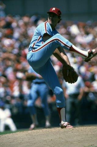
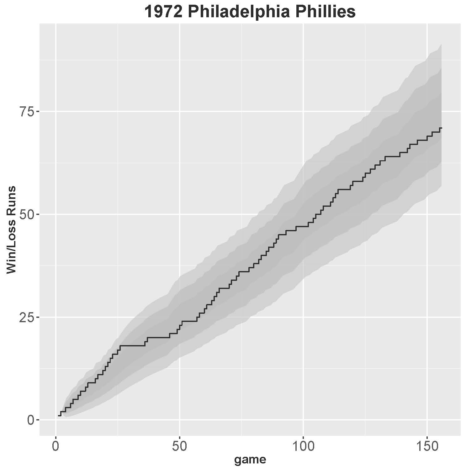
To understand how we compute the runs statistic, consider the win-loss data from the 1972 Philadelphia Phillies. We did not choose this Phillies team randomly; this team was known not only for being a bottom-rung team, but one that had a pitching ace, Steve Carlton, who finished with a 27–10 record in 41 starts, with a 1.97 ERA. The other three main starting pitchers on the team had a combined 10-39 record, and Carlton earned nearly half the team’s wins that season.

For that reason, one might conjecture the 1972 Phillies would have a peculiar kind of streakiness: abbreviated winning streaks along with longer losing streaks that were halted when Carlton was the starting pitcher. In fact, this happened 19 times when a Phillies loss was followed by a winning game started by Carlton. But in the course of the year, we will see that peculiarity did not give the Phillies an unusual pattern of losing streaks that were truncated at four or so games. Overall, we will show the Phillies team was no streakier than we would expect from a team that has the same 37.8% chance of winning any game.

Here is how the 1972 Philadelphia Phillies season is summarized in terms of daily wins (W) and losses (L):

WLLWWLWWLWWLWWWLWWL
WLWLLWLLLLLLLLLLWLLLLLLLLL
WWWLWLLLLLLWLLWLLWLWLLLL
WLLWLLLLWWLLWLLWLLWLWWW
LLLLWWWWWLLWLLWLLLWLW
LLLLLWLLLLWLLWWLLWWLLLLLL
WWWLWWWLLLLWWLLLWW

For example, the first streak is a winning streak, which lasts only one game. The next streak must be a losing streak, which lasted two games.

 

(Click image to enlarge.)

 

Figure 1 plots these streak sequences for the 1972 Phillies as a step function, stepping up each time a new streak starts. The flat part in the line that starts at 25 games represents a 10-game losing streak the Phillies began on May 16, and ended with a win on May 27. The step function will jump over and up with apparent randomness, but if the final statistic (after 162 games) ends up within the darkest gray (middle) region, then the runs statistic is within one standard deviation of the number of runs we would expect if the sequence was based on random Bernoulli trials. By graphing the path of the runs statistics, we are able to assess when and why a team’s streaks were notable. In this particular case, the final number of runs (for a 59–97 team) is well within the expected bounds we would expect if the Phillies had the same probability of winning each game (e.g., 59/156 = 0.378. Note that only 156 games were played due to the strike.).

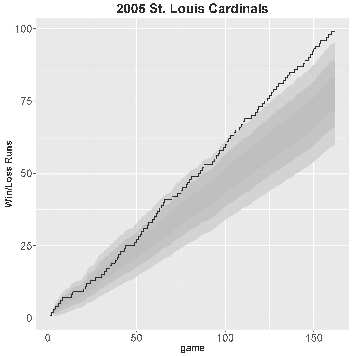
The runs test will signal non-randomness (a potential streaky sequence) if the plotted step function ends up outside two standard deviations after 162 games. The two standard deviation interval is represented by the second, slightly lighter gray band in Figure 1. The lightest band represents a runs statistic within three standard deviations. If the win-loss sequence is truly random, we would expect a team to fall outside three standard deviations once every 370 seasons. In terms of our accumulated data across 55 years, that is equivalent to saying we would expect to see 3.93 teams experience having a runs statistic more than three standard deviations from the expected value. We actually found only one such team matching a standard deviation over three—the 2005 St. Louis Cardinals (discussed below). We also found 94.5% of the runs statistics were within two standard deviations, which is very close to what would be expected if there is no streakiness. 

2005 ST. LOUIS CARDINALS

As the sole outlier in over 50 years of accumulated data, the 2005 St. Louis Cardinals are worthy of extra scrutiny. In that year, the Cards went 100–62 (but lost to the Houston Astros in the National League Championship Series). They were led by 25-year-old first baseman Albert Pujols, who garnered 41 home runs, 117 RBIs, and batted .330. Chris Carpenter led the pitching staff with a 21–5 record and a 2.83 ERA. What made this team’s runs sequence exceptional is not the long winning streaks, but the lack of losing streaks.

The Cardinals recorded 99 streaks (50 winning streaks and 49 losing streaks). The table below shows that St. Louis stopped losing streaks at one game 39 times, which is over 30% more frequent than expected for a team with a 0.617 winning average. That is, if we observe 49 independent random trials representing the number of games (after their initial loss) until they win a game, then the probability the streak ends on the next game is 0.617, which should happen (0.617)49 = 30.2 times out of 49. For the 2005 St. Louis Cardinals, the losing streak ended after one game 39 out of 49 times. 

 

Table 1

Streak	1	2	3	4	5	6
WIN	24	14	6	2	3	1
expected	19.1	11.8	7.3	4.5	2.8	1.7
LOSS	39	7	3	0	0	0
expected	30.2	11.6	4.4	1.7	0.6	0.2

 

Figure 2 shows how the Cards’ season became less streaky as the season progressed. The Cardinals’ year of 99 streaks is among the highest recorded over the past 55 years, but the highest number of streaks—100—belongs to the 1971 California Angels. The Angels had a mediocre record of 76–86 but had fewer than expected long streaks of wins or losses. Out of 50 winning streaks, 34 were ended after one game (much higher than the 23.5 expected).

 

(Click image to enlarge.)

 

2003 DETROIT TIGERS

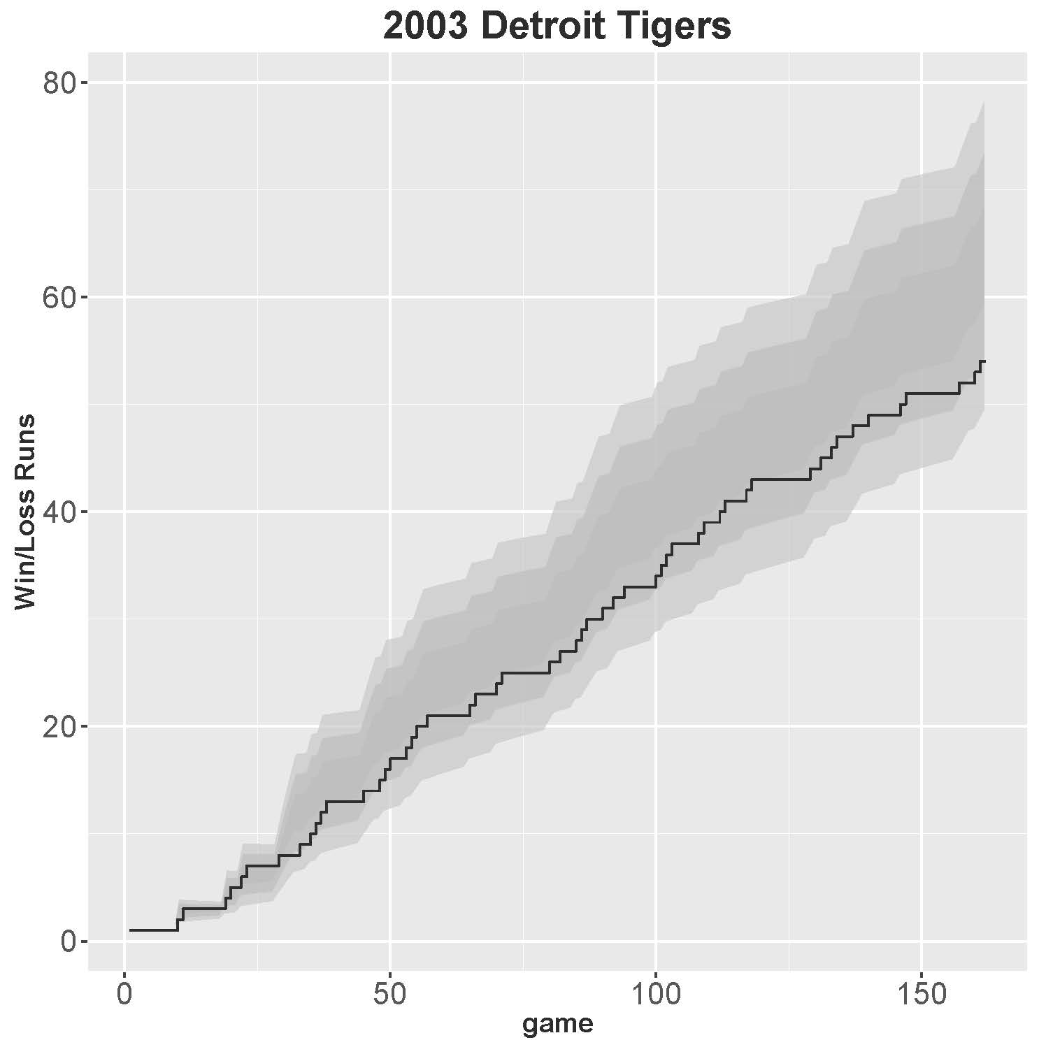
The streakiest team of the past 55 years is the 2003 Detroit Tigers, one of the worst teams in major league baseball history. The Tigers compiled a record of 43–119, breaking a record for AL teams by recording more losses than the 1916 Philadelphia Athletics. With 27 winning streaks and 27 losing streaks, the Tigers had the fewest number of streaks of all major league teams since 1962, not counting the 1981 and 1994 strike-shortened seasons. Figure 3 shows how their accumulation of streaks developed over the season.

For a team with a 43–119 record, long losing streaks are inevitable. If we treat each game as an independent trial, then we would expect 27(0.2654)=7.2 losing streaks that would end at one game (actually, 6 streaks ended at one game). On the other hand, we would expect between two and three losing streaks of six games or more. In 2003, the Tigers endured ten different losing streaks of six or more games, including a 10-game losing streak in September and an 11-game losing streak in August. These long streaks account for why the ’03 Tigers runs statistic is such an aberration. In the seven losing streaks of seven or more games, the Detroit Tigers accumulated more than half of their losses for the season (62 out of 119).

 

(Click image to enlarge.)

 

Table 2

Streak	1	2	3	4	5	6
WIN	17	5	4	1.7	0	0
expected	19.8	5.3	1.4	0.4	0.1	0
LOSS	6	4	4	2	1	3
expected	7.2	5.3	3.9	2.8	2.1	1.5
Streak	7	8	9	10	11
WIN	0	0	0	0	0
expected	0	0	0	0	0
LOSS	1	2	2	1	1
expected	1.1	0	0	0	0

 

CONCLUSIONS

Once any non-random pattern is determined from a runs test, more advanced statistical methods may be used to characterize how each team’s win probability changes depending on whether the last game is a win or a loss.  In related research, Quintana, et al. analyzed individual batters’ streakiness with regard to hits, and looked at how a player’s performance varied from season to season (across four seasons).[fn]Quintana, F.A., Muller, P., Rosner, G.L., and Munsell, M. (2008). “Semiparametric Bayesian Inference for Multi-Season Baseball Data,” Bayesian Analysis, 3: 317–38.[/fn] Some obvious factors were helpful in predicting how a player’s success rate might change, such as the quality of the opposing pitcher, but for the most part, explanatory variables such as game score or inning were not helpful in the prediction.

According to the distribution of the nonparametric Wald-Wolfowitz runs test, we found close to the expected number of results within one and two standard deviations of what was expected. Interestingly, we found fewer than expected cases outside of three standard deviations. Obviously, the simplicity of the applied runs test does not reveal the subtle win probability factors that change from day to day, from series to series, from pitching match up to who is on the disabled list. But the data show that detailed investigations into team streakiness are not warranted due to the overwhelming evidence that winning streaks and losing streaks fall into a pattern that is consistent with independent, random trials.

PAUL KVAM is professor of Mathematics and Statistics at University of Richmond. Kvam is author or co-author of several sports-related statistics papers, including “Comparing Hall of Fame Baseball Players Using Most Valuable Player Ranks” (2011), “A Logistic Regression/Markov Chain Model For NCAA Basketball” (2006), and “Teaching statistics with sports examples” (2005).

ZEZHONG CHEN is a graduate student at Cornell Tech in New York City.