A Truer Measure of ‘Games Behind’

Baseball fans know that games behind (GB), the number that appears in the last column of each     day’s standings, is not always an accurate measure of the distance between two teams. GB is the average of the number of games a team trails the percentage leader in the win column and the number of games that team trails the leader in the loss column. To illustrate, consider the major league standings at the All-Star break in 1985:

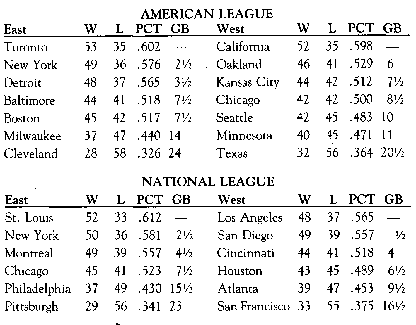
In the American League West, Oakland trailed California by 6 in the win column and by 6 in the loss column, so Oakland was 6 games behind. In the East, however, New York trailed Toronto by 4 in the win column and by 1 in the loss column; these averaged to 2½ games behind.

In the National League East, New York trailed St. Louis by 2 in the win column and 3 in the loss column, so the Mets were 2½ games behind the Cardinals. In the West, San Diego, although trailing in percentage, was actually one win ahead of Los Angeles (so the Padres “trailed” by – 1) while trailing by 2 in the loss column, which meant San Diego was ½ game behind Los Angeles because ½ is the average of – 1 and 2.

There are two problems with using GB as a measure of the distance between the trailing team and the leader. The first is illustrated by the following hypothetical standing. You’ll note the Trailers “trail” by -4 in the win column and by 3 in the loss column. Thus the Trailers are – ½ game “behind” the Leaders – that is, the Trailers are ½ game ahead of the Leaders, even though they have a lower percentage. Here’s the standing:

  Leaders             18        13   .581   ½

  Trailers             22        16   .579   —

The second problem is reflected in the fact that baseball players and the media always qualify their assessment of games behind with a reference to the “all-important loss column.” For example, in the 1985 standings that we looked at, both New York teams were 2½ games behind, but were they really the same distance from their respective leaders? Most fans would say that the Yankees were closer to the Blue Jays than the Mets were to the Cardinals because the Yankees were only one behind in the loss column while the Mets were three behind in the loss column. If the Blue Jays lost one more game, the Yankees would have been able to achieve at least a tie for first place by winning all their “remaining” games; in baseball’s cliche, they would “control their own destiny.” By contrast, the Mets would not have been in such a position unless the Cardinals lost three games.

There is a different way of calculating the distance between teams that avoids both of these problems. Let’s call it the deficit between the teams in order to avoid confusion with games behind. By definition, the deficit between two teams is a number D such that if the trailing team won D games and the leading team lost D games, they would have the same winning percentage.

Let’s calculate D for each second-place team in the standings listed earlier in this article. The easiest calculation is for Oakland. If Oakland won D more games and California lost D more, the standings would read:

  California        52                     35  +   D

  Oakland           46  +       D       41

It’s obvious the solution is D = 6 because both teams would then have records of 52-4 1. Thus, deficit and games behind are equal when the teams have played the same number of games.

  The other divisions are more complicated. In the

American League East, if the Yankees’ deficit is D, then the Blue Jays and Yankees would be tied if the standings were:

  Toronto         53                 35  +   D

  New York        49 +   D     36

Thus, D is the solution to the equation   

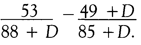
Solving by cross-multiplication we get

53(85 + D) = (88 + D) (49 + D)

4505 +53D = 4312 +88D + 49D + D²

0 = D² + 84D – 193.

This is a quadratic equation, which can be solved easily with a calculator, using the quadratic formula. (The quadratic formula says: If  ax2 + bx + c = 0, then x =  

Don’t worry if you don’t know it; we’ll give a practical algorithm for calculating D later.) The solution, rounded to two decimal places, is D = 2.24. Thus the deficit between the Yankees and the Blue Jays was 2.24 games. This confirms our intuition that the Yankees were actually less than 2½ games behind because they were only 1 behind in the loss column. Note that if such a thing were possible and the Yankees won 2.24 more games and the Blue Jays lost 2.24 more games, the standings would read:

  New York        51.24    36        .587

  Toronto            53         37.24   .587

So the teams would be tied. (The tie is not exact because we rounded D to two decimal places.)

Earlier we said we thought the Mets were farther behind the Cardinals than the Yankees were behind the Blue Jays because the Mets trailed the Cardinals by 3 in the loss column. Watch what happens when we calculate the Mets’ deficit:

  St. Louis        52              33  +   D

  New York      50  +         D   36

By the quadratic formula, D = 2.59. So it’s true that the Mets were really more than 2½ games behind the Cardinals.

Finally, let’s calculate the Padres’ deficit with respect to the Dodgers. If the Padres won D more games and the Dodgers lost D more games, the standings would read:

  Los Angeles      48            37  +   D

  San Diego        49  +          D   39

So by the quadratic formula, D = 0.68. Thus the Padres were really more than ½ game behind the Dodgers, which is what we expected because they trailed by 2 in the loss column.

Here is the formula for calculating D:

1. Let A and B denote the numbers of wins and losses for the leading team and let a and b denote the number of wins and losses for the trailing team.

2. Let P = B + a, the sum of the leading team’s losses and the trailing team’s wins.

3. Let Q = Ab – Ba, the product of the leading team’s wins and the trailing team’s losses minus the product of the leading team’s losses and the trailing team’s wins.

4. Square P (multiply it by itself).

5. Multiply Q by 4 and add this to the previous result.

6. Take the square root of this number.

7. Subtract P.

8. Divide by 2 and round off to two decimal places.

It’s obvious that D is more difficult to calculate than GB, but it still takes only a few seconds on a calculator. It would be simple to write a computer program that would calculate percentages and deficits on the basis of given won-lost records. Thus, we need not, in the present high-tech age, sacrifice the precision of D for the computational simplicity of GB. Here are the major league standings at the All-Star break of the 1985 season as they would look with deficit in place of games behind:

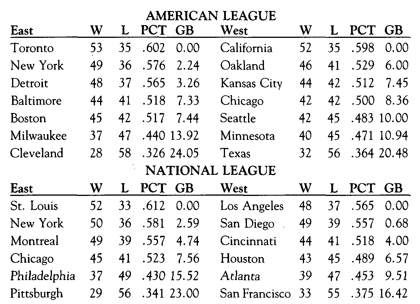
Compare the standings showing deficit with the standings showing games behind. The deficits reveal that the Yankees were closer to first place in their division than the Mets were in theirs, as was noted.

One more important fact about deficit: The anomalous situation described earlier, in which a team trailing in percentage is actually ahead of the leader in terms of games behind, cannot occur. We’ll leave it as an exercise for the reader to calculate the deficit between the Trailers and the Leaders.