Appendix 1: Analysis of Andrés Galarraga’s Home Run of May 31, 1997

This is the appendix for “Analysis of Andres Galarraga’s Home Run of May 31, 1997,” by José L. López, Oscar A. López, Elizabeth Raven, and Adrián López.

Editor’s note: This is the appendix for “Analysis of Andres Galarraga’s Home Run of May 31, 1997,” by José L. López, Oscar A. López, Elizabeth Raven, and Adrián López.

This appendix describes in detail the procedure followed to obtain the most reliable solutions for the Galarraga’s home run. To select them, the maximum height (H) reached by the ball in each of the 18 trajectories obtained is compared to the height shown in the video after performing orthogonal and conical projections. Figure A1 (top) shows a plan view of the stadium obtained from LIDAR point clouds using the program Global Mapper. Home plate, the ball’s point of impact, and the location of the camera were plotted on this plan.

 

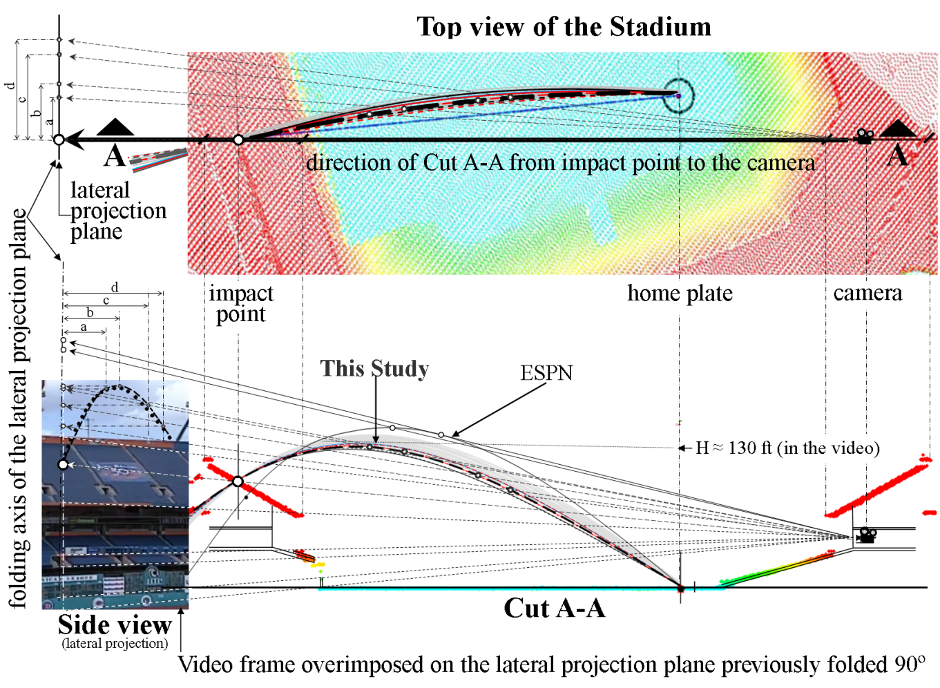
Figure A1. Plan and cut of the stadium obtained from the LIDAR image showing a conical projection of the 18 trajectories and some significant points. Top: Plan view indicating cut A-A which goes from the camera to the impact point (Row 20). Bottom: Vertical view through cut A-A. (Click image to enlarge.)

 

Cut A-A in Figure A1 (bottom), also made using the LIDAR point clouds, shows a side view of the stadium and it passes through the location of the camera and the ball’s point of impact. Note the colored points of LIDAR in Figure A1 (bottom) that delineate the right sector of the stadium where the press box and the camera are plotted as well as the left sector where the ball hit row 20. The 18 trajectories are also shown in the figure; the dark lines indicate the 7 most reliable solutions (Table 2) and the lighter lines indicate the remaining 11 solutions.

Figure A2 shows an enlargement of the lower portion of Figure A1. Only the 7 most reliable solutions (Table 2) are shown in Figure A2. For comparison purposes the solution proposed by ESPN (2016) is also shown.

 

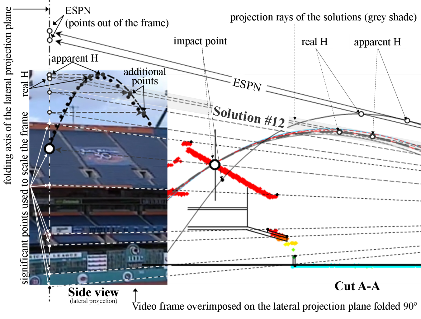
Figure A2. Comparison of the trajectories and maximum heights drawn on the video frame showing the maximum heights (H) of the seven most reliable solutions found by this study and the one found by ESPN Home Run Tracker (2016). (Click image to enlarge.)

 

Conical projections are shown in the top and side views of Figure A1. Several rays go from the focus located in the camera to the lateral projection plane shown at the left end of figures A1 and A2. Those rays pass through several points such as the ball’s point of impact, the maximum heights of the trajectories and significant points of the stadium, as indicated.

For visualization purposes this lateral projection plane is folded 90 ° along its axis and shown at the left end of figures A1 and A2 where a video frame is superimposed. The video frame shows the stadium from the bottom to the top. In order to correctly scale the video frame with the orthogonal projections, its size is adjusted using the rays previously mentioned so that they match some characteristic points of the stadium such as border of railing of the stands. These rays also pass through the highest points of the trajectories (real and apparent H) and by the point of impact, extending to the lateral plane of projection, as pointed out in Figure A1 (bottom) and Figure A2. A 3D view of the conical projection, made using a SketchUp pre-existing model of the stadium (3D Warehouse, 2016), can be seen in Figure A3 where one solution is used as an example of the procedure.

 

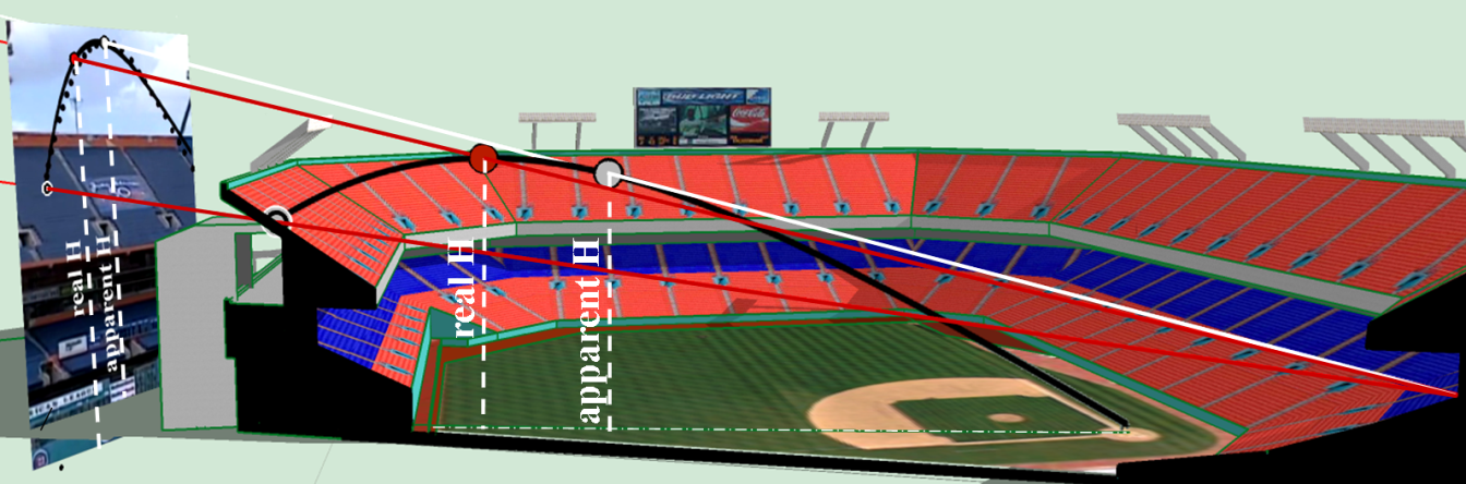
Figure A3. Real and apparent maximum height H. Right: in the 3D model the real H is higher than the apparent H. Left: in the video frame the apparent H looks higher than the real H due to an optical effect induced by the inclination angle of the camera. (Click image to enlarge.)

 

For the discussion that follows, it should be kept in mind that in the video the ball at its highest point is always shown within the frames throughout the filming, i.e. the cameraman never lost sight of the ball until the moment it impacted the deck. In Figure A2 the maximum height indicated by the video frame can be compared to the maximum heights of the solutions found.

A geometric analysis was done for the eighteen solutions (Table 2) but only seven are shown in Figure A2 because they have maximum heights within the video frame as indicated by the grey shade superimposed to the projection rays of the maximum heights; the other solutions were discarded because they reached heights that were outside of the video frame and therefore are not considered reliable solutions. ESPN’s maximum height is also outside the video frame as shown on the same figure. As a result, the most reliable solutions whose maximum heights remain inside the video are the following: Solutions #5 and #6 for wind hypothesis 1, solutions #11 and #12 for wind hypothesis 2 and solution #16, #17 and #18 for wind hypothesis 3. These are highlighted in Table 2. At this point it is important to explain that Figure A2 indicates two maximum heights for each solution: the real maximum height (real H) which is represented by the top point of the ball’s trajectory and the apparent maximum height (apparent H) which is represented by the tangent point of the trajectory with a projection line that goes from the camera to the lateral plane. The apparent H appears to be in the video higher than the real H but actually is not as can be seen in Figure A3, where a 3D view of the trajectory of one solution is shown. This figure clearly shows which one is the real maximum height (real H). This optical effect occurred because the location of the camera was low and close to the home plate. As a consequence, the maximum height of the ball in the video seems to occur 2.5 seconds after the ball is impacted by the bat, when in fact happens around 3.0 and 3.1 seconds as predicted by the model and as indicated in the seven most reliable solutions in Table 2.

The ball’s impact point, the actual ball trajectory taken from the video (black dots) and the trajectory of Solution #12 (black dashed line), were projected and drawn on the video frame shown to the left in Figure A2. This solution is taken as an example from the seven most reliable solutions.

The dots at the top of the actual ball’s trajectory are a portion of the trajectory that couldn’t be seen in the video due to the clouds; this portion was estimated by interpolation with the video editing software (Adobe Premiere).

Five points were used to project solution #12: impact point, real H, apparent H and two additional points that allowed its interpolation, as shown in Figures A1 and A2. The similarities between the ball’s trajectory #12 (black dashed line) and the actual trajectory from the video (black dots) can be seen in Figure A2, which validate the solution.