

RBI, Opportunities, and Power Hitting: Opportunities Significantly Affect RBI Totals
This article was written by Cyril Morong
This article was published in 2002 Baseball Research Journal
RBI have long been one of the staples of measuring a hitter’s contribution to his team’s success. Sometimes a player is said to be “a good RBI guy.” Newspapers and record books list the annual RBI leaders, scoreboards and broadcasters tell us how many RBI a hitter has, almost as if getting them is a special skill, separate from power hitting or hitting for average. But RBI are also often criticized as being misleading since all hitters don’t get the same number of opportunities to drive in runs. One hitter might get more RBI than another because he had more opportunities and not because he is somehow better at driving in runs. So the important question is: Exactly how much difference do RBI opportunities make?
They make a big difference and exactly how big can be learned from statistical analysis. The following equation, derived using the linear regression technique, explains a hitter’s RBI per at-bat and the value of opportunities:
EQUATION 1
RBI / AB = .125 x OPP + .194 x AVG + .514 x ISO – .20
where
- OPP = number of RBI opportunities per at-bat
- AVG = batting average
- ISO = isolated power
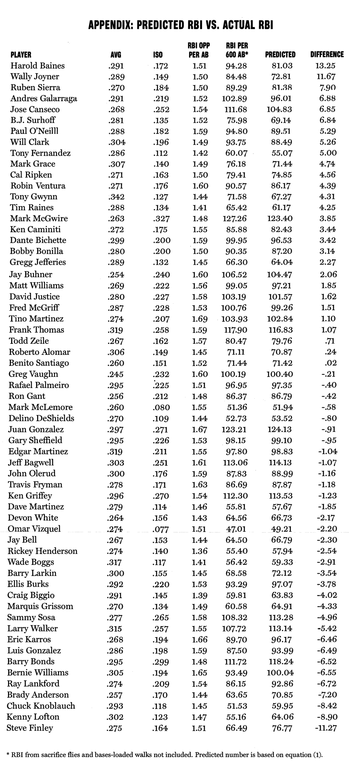
How does this work? Equation 1 predicts that Juan Gonzalez would get .206 RBI per at-bat because:
.125 x (1.67) + .194 x (.297) + .514 x (.271) – .20 = .206
Gonzalez actually had .205 RBI per at-bat. The equation is also generally very accurate (I explain the statistical results and the data below).
But first, what does the equation mean from a baseball perspective? With the coefficient on OPP being .125, two players who differ by, say, .15 OPP (90 RBI opportunities for a 600 at bat season), will end up with an 11.28 difference in RBI over a 600 at-bat season (11.28 = .15 x .125 x 600).
This is significant in baseball terms as well as statistically. Why look at a .15 difference in OPP? This study includes all players (61) who had 6,000 or more plate appearances during the 1987-2001 seasons and whose situational statistics were listed on the CNN/SI Web site.1 Tino Martinez had the highest OPP/AB at 1.69 for his career. More than half of the other players were at least .15 less than this, including other power hitters like Jose Canseco, Ken Griffey Jr., and Gary Sheffield. Barry Bonds was even lower at 1.48. Martinez would get 15.79 (or .21 x .125 x 600) more RBI than Bonds solely as a result of having more opportunities.
For a single season, the differences in OPP can be even greater. In 1995 for example, Paul O’Neill was the leader at 1.85 while Barry Bonds had 1.61. Everything else being equal, O’Neill would get about 18 more RBI over a 600 at-bat season. So opportunities play a big role in RBI totals.
Hitters vary quite a bit in RBI opportunities. For example, the two lowest in OPP/AB were Rickey Henderson and Craig Biggio, at 1.36 and 1.39, respectively. The two highest were Juan Gonzalez and Tino Martinez at 1.67 and 1.69, respectively. Of course, Henderson and Biggio are both primarily leadoff men while Gonzalez (usually fourth) and Martinez (usually fifth or sixth) have been largely used in the middle of the lineup. But the difference between Rickey and Tino (.33 OPP) would be 198 more RBI opportunities over the course of a 600 at-bat season. Just bout half of that, say .15, would mean about 90 more.
An actual example supports the importance of opportunities. Juan Gonzalez has a career average of .297 and an ISO of .271. Ken Griffey Jr. had .296 and .270, almost identical numbers. Yet Gonzalez had .205 RBI/AB or 123 RBI over a 600 at-bat season. Griffey had .187 RBI/AB or 112 over a 600 at-bat season. The difference results from Gonzalez having 1.67 opportunities per at-bat while Griffey had 1.54.
As for the data, opportunities include one for every time at bat and one for each runner on base during an at-bat. This means that OPP does not include opportunities from plate appearances when the batter walked. (A regression was run that included these opportunities, and the results were similar).2 Isolated power is a hitter’s slugging percentage minus his batting average and is a better measure of power hitting since it only includes bases on hits beyond singles.
As for the statistical results, the r2 is .943, which means that 94.3% of the difference in RBI per at-bat across players is explained by Equation 1. The standard error, which measures dispersion in the equation’s predicted RBI/AB for each player, is .00839 or just 5.03 RBI for a 600 at-bat season (600 x .00839 = 5.03). The numbers in front of the variable abbreviations are referred to as coefficient estimates. So, for example, a .010 increase in batting average means a .00194 increase in RBI/AB (.194 x .010 = .00194).
That is 1.16 RBI for a 600 at-bat season. A .010 increase in ISO would add 3.08 RBI for a 600 at-bat season. The T values, which indicate statistical significance, are:
- OPP = 7.25
- AVG = 3.35
- ISO = 22.25
This says that the three variables are all significant at the 1% level (or lower), meaning that there is less than a 1 in 100 chance of getting the coefficient estimates in Equation 1 if their true value were zero.
Equation 1 also shows the bigger role played by power hitting in driving in runs. Consider Players A and B, who have the following statistics:
| PLAYER | AB | H | 2B | 3B | HR | AVG | SLG | ISO |
| A | 600 | 192 | 40 | 8 | 16 | .320 | .493 | .173 |
| B | 600 | 162 | 20 | 4 | 32 | .270 | .477 | .207 |
Who will drive in more runs? Using Equation 1 and assuming they each get 1.5 OPP, Player A will drive in 83.2 runs while Player B will drive in 87.66 runs. Player B’s edge in home run power gives him the edge in RBI despite a much lower batting average and a deficit in doubles and triples. For Player A to get up to 87.66 RBI, his average would have to jump to .358 (assuming all additional hits are singles). If Player A had just 20 doubles and 4 triples, along with a .320 average, he would drive in just 68.8 runs. To get up to 87.66 RBI, he would then have to raise his average to .482! (Again, assuming additional hits are singles.)
But are all RBI opportunities of the same quality? No, a runner on third is better than a runner on first. So a runner on third counted as a four-point opportunity, a runner on second as a three-point opportunity, a runner on first a two-point opportunity, and the batter as a one-point opportunity. So I ran another linear regression with points per at-bat replacing opportunities per at-bat.
The following equation shows the results:
EQUATION 2
RBI/AB = .069 x PTS + .212 x AVG + .479 x ISO – .18
The r2 is .969. The standard error is .00614 or just 3.68 RBI for a 600 at-bat season. This result is even better than the one summarized in Equation 1. Notice that the value of ISO is still much greater than the value of average, so power hitting is still the dominant force. The three variables were all statistically significant at the 1% level. Equation 2 is very accurate, predicting to within six RBIs per 600 at-bats for 56 of the 61 hitters. Also, a regression was run that included opportunities from walks, as converted into points, with similar results.
What do these results mean in baseball terms? With the value of PTS being .069, two players who differ by, say, .30 PTS, will end up with a 12.36 difference in RBI for a 600 at bat season (12.36 = .3 x .069 x 600). This is significant in baseball terms as well as statistically. Why look at a .3 difference in PTS? Juan Gonzalez had the highest, at 2.85. About half the players in the study were below 2.55. Barry Bonds, for example, had 2.4. So with equal hitting performances, Juan Gonzalez would get 18.5 (or .45 x .069 x 600) more RBI than Bonds solely as a result of having more opportunities and better quality opportunities.3
A hitter’s RBI are determined by his ability to hit for average, hit for power and the quality and quantity of his opportunities. There probably is no special “RBI ability.” The vast majority of hitters will get about the number of RBI predicted by their general hitting ability and opportunities. Any deviations are probably just random chance. That would be consistent with the well-known research on clutch hitting.
CYRIL MORONG is a professor of economics at San Antonio College in San Antonio, TX. He is originally from Chicago and is a lifelong White Sox fan.
APPENDIX 1: PREDICTED RBI VS. ACTUAL RBI
SOURCES
Various editions of the STATS, Inc. Player Profiles books and The Great American Baseball Stat Book.
Brooks, Harold. “The Statistical Mirage of Clutch Hitting,” Baseball Research Journal, 1989.
Conlon, Tom. “Or Does Clutch Ability Exist?” By The Numbers, March 1990.
Cramer, Richard D. “Do Clutch Hitters Exist?” Baseball Research Journal, 1977.
Gillette, Gary. “Much Ado About Nothing,” Sabermetric Review, July 1986.
Hanrahan, Tom. “What Makes a “Clutch” Situation?” By the Numbers, February 2001.
Karcher, Keith. “The Power of Statistical Tests,” By The Numbers, June 1991.
Mills, Eldon G. and Harlan D. Mills. Player Win Averages, New York: A.S. Barnes, 1977.
Palmer, Pete. “Clutch Hitting One More Time,” By the Numbers, March 1990.
Runquist, Willie. “Clutch Hitters and Other Mythological Animals,” Baseball by The Numbers, Jefferson, NC: McFarland, 1995.
Wood, Rob. “Clutch Ability: Myth or Reality?” By the Numbers, December 1989.
NOTES
1. Some outstanding hitters of recent times, Manny Ramirez and Mike Piazza, for example, were not in the study since they had not achieved 6,000 plate appearances through the 2001 season. Both were high in opportunities per at-bat at 1.71 and 1.68, respectively. Ramirez had about .5 more RBI per 600 at-bats than expected and Piazza had about .26 less.
2. RBI from sacrifice flies are also not included. Neither are opportunities that were available when the player hit a sacrifice fly. For the average player in this study, sacrifice flies make up less than 1 % of his plate appearances and no more than 1.5% for any one player. So excluding sacrifice flies matters very little. RBI from bases-loaded walks were not included in the Equation 1 or Equation 2 results. They were included in the unreported regressions that included opportunities from walks. In those regressions, all variables were divided by plate appearances rather than at-bats. HBPs were also included in those cases. But again, the results were similar with basically the same meanings as the two regressions reported here.
3. If I used walks, plate appearances, and the point system, the regression results show that opportunities alone would give Juan Gonzalez 15 more RBI than Barry Bonds over a 660 plate appearance season. That is less than 18.5, but still very high.