

Runs and Wins
This article was written by Pete Palmer
This article was published in The National Pastime: Premiere Edition (1982)
This article was selected for inclusion in SABR 50 at 50: The Society for American Baseball Research’s Fifty Most Essential Contributions to the Game.
Most statistical analyses of baseball have been concerned with evaluating offensive performance, with pitching and fielding coming in for less attention. An important area that has been little studied is the relationship of runs scored and allowed to wins and losses: how many games a team ought to have won, how many it did win, and which teams’ actual won-lost records varied far from their probable won-lost records.
The initial published attempt on this subject was Earnshaw Cook’s Percentage Baseball, in 1964. Examining major-league results from 1950 through 1960 he found winning percentage equal to .484 times runs scored divided by runs allowed. (Example: in 1965 the American League champion Minnesota Twins scored 774 runs and allowed 600; 774 times .484 divided by 600 yields an expected winning percentage of .630. The Twins in fact finished at 102-60, a winning percentage of.624. Had they lost one of the games they won, their percentage would have been .623.) Arnold Soolman, in an unpublished paper which received some media attention, looked at results from 1901 through 1970 and came up with winning percentage equal to .102 times runs scored per game minus .103 times runs allowed per game plus .505. (Using the ’65 Twins, Soolman’s method produces an expected won-lost percentage of.611.) Bill James, in his Baseball Abstract, developed winning percentage equal to runs scored raised to the power x, divided by the sum of runs scored and runs allowed each raised to the power x. Originally, x was equal to two but then better results were obtained when a value of 1.83 was used. James’ original method shows the ’65 Twins at .625, his improved method at .614.)
My work showed that as a rough rule of thumb, each additional ten runs scored (or ten less runs allowed) produced one extra win, essentially the same as the Soolman study. However, breaking the teams into groups showed that high-scoring teams needed more runs to produce a win. This runs-per-win factor I determined to be equal to ten times the square root of the average number of runs scored per inning by both teams. Thus in normal play, when 4.5 runs per game are scored by each club, the factor comes out equal to ten on the button. (When 4.5 runs are scored by each team scores .5 runs per inning –totally one run, the square root of which is one, times ten.) In any given year, the value is usually in the nine to eleven range. James handled this situation by adjusting his exponent x to be equal to two minus one over the quantity of runs scored plus runs allowed per game minus three. Thus with 4.5 runs per game, x equals two minus one over the quantity nine minus three: two minus one-sixth equals 1.83.
Based on results from 1900 through 1981, my method or Bill’s (the refined model taking into account runs per game) work equally well, giving an average error of 2.75 wins per team. Using Soolman’s method, or a constant ten runs per win, results in an error about 4 percent higher, while Cook’s method is about 20 percent worse.
Probability theory defines standard deviation as the square root of the sum of the squares of the deviations divided by the number of samples. Average error is usually two-thirds of the standard deviation. If the distribution is normal, then two-thirds of all the deviations will be less than one standard deviation, one in twenty will be more than two away, and one in four hundred will be more than three away. If these conditions are met, then the variation is considered due to chance alone.
From 1900 through 1981 there were 1448 team seasons. Using the square root of runs per inning method, one standard deviation (or sigma) was 26 percentage points. Seventy teams were more than 52 points (two sigmas) away and only two were more than 78 points (three sigmas) off. The expected numbers here were 72 two-sigma team seasons and 4 three-sigma team seasons, so there is no reason to doubt that the distribution is normal and that differences are basically due to chance.
Still, it is interesting to look at the individual teams that had the largest differences in actual and expected won-lost percentage and try to figure out why they did not achieve normal results. By far the most unusual situation occurred in the American League in 1905. Here two teams had virtually identical figures for runs scored and allowed, yet one finished 25 games ahead of the other! It turns out that with one exception, these two teams had the largest differences in each direction in the entire period. Detroit that season scored 512 runs and allowed 602. The Tigers’ expected winning percentage was .435, but they actually had a 79-74 mark, worth a percentage of .517. St. Louis, on the other hand, had run data of 511-608 and an expected percentage of .430, yet went 54-99, a .353 percentage.
Looking at game scores, the difference can be traced to the performance in close contests. Detroit was 32-17 in one-run games and 13-10 in those decided by two runs. St. Louis had marks of17-34 and 10-25 in these categories. Detroit still finished 15 games out in third place, while St. Louis was dead last. Ty Cobb made his debut with the Tigers that year, but did little to help the team, batting .240 in 41 games.
The only team to have a larger difference between expected and actual percentage in either direction than these two teams was in the strike-shortened season last year, when Cincinnati finished a record 88 points higher than expected. Their 23-10 record in one-run games was the major factor. The 1955 Kansas City Athletics, who played 76 points better than expected, had an incredible 30-15 mark in one-run games, while going 33-76 otherwise.
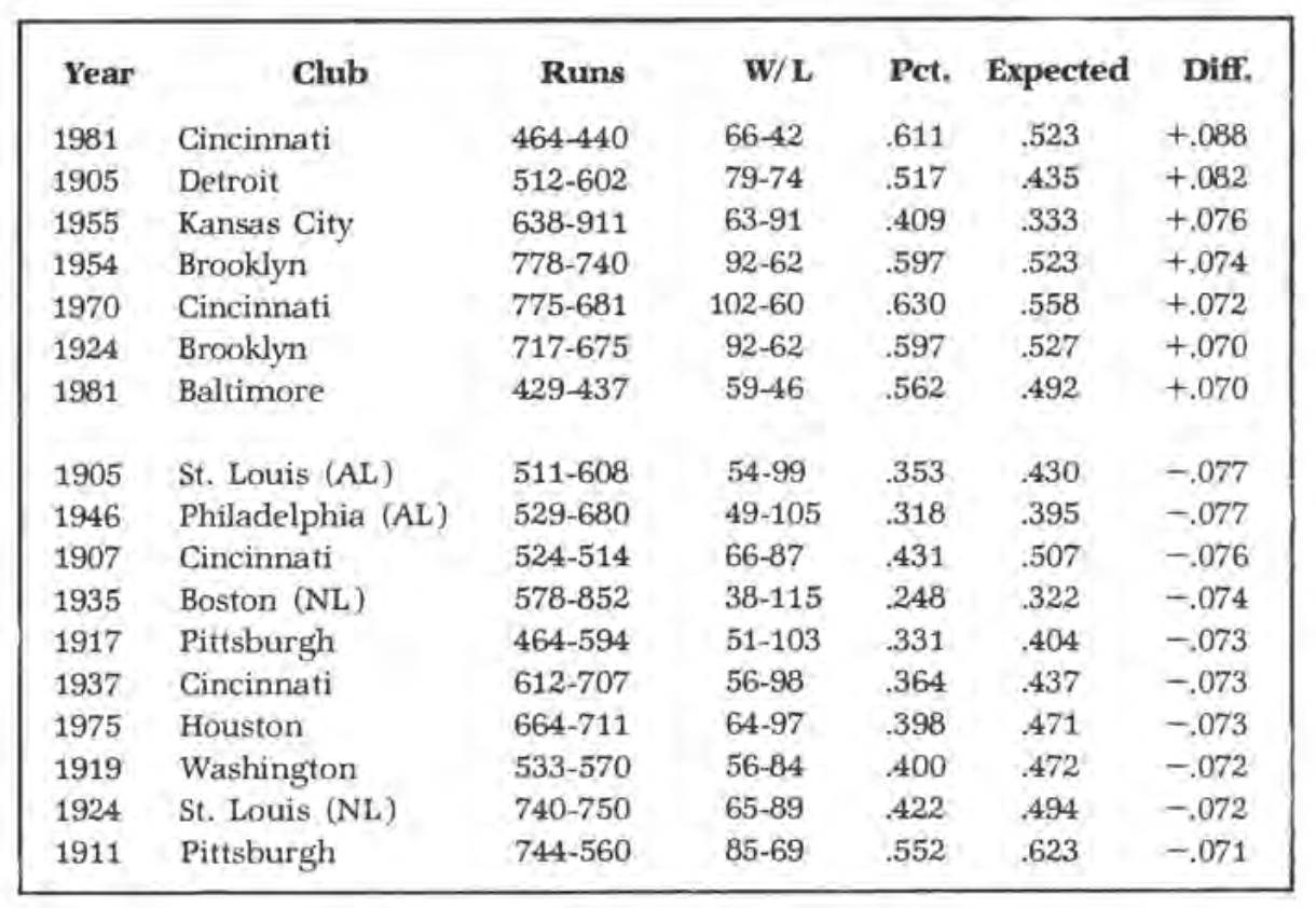
(Click image to enlarge)
Listed above are all the teams with differences of 70 or more points.
The 1924 National League season affords an interesting contrast which is evident in the chart. St. Louis failed of its expected won-lost percentage by 72 points while Brooklyn exceeded its predicted won-lost mark by 70.
The two poor showings by the Pittsburgh club in 1911 and 1917 were part of an eight-year string ending in 1918 in which the Pirates played an average of 37 points below expectations, a difference of about six wins per year. This was the worst record over a long stretch in modern major-league history. Cincinnati was 40 points under in a shorter span, covering 1902 through 1907. No American League team ever played worse than 25 points below expectation over a period of six or more years.
On the plus side, the best mark is held by the current Baltimore Orioles under Earl Weaver. From 1976 through 1981 they have averaged 41 points better than expected. The best National League mark was achieved by the Brooklyn and Los Angeles Dodgers in 1954-63, 27 points higher than expectations over a ten-year period, or about four wins per year.
The three-sigma limit for ten-year performance is 25 points. The number of clubs which exceeded this limit over such a period is not more than would be expected by chance. So it would seem that the teams were just lucky or unlucky, and that there are no other reasons for their departure from expected performance.
Here are the actual results and differences for the four teams covered.
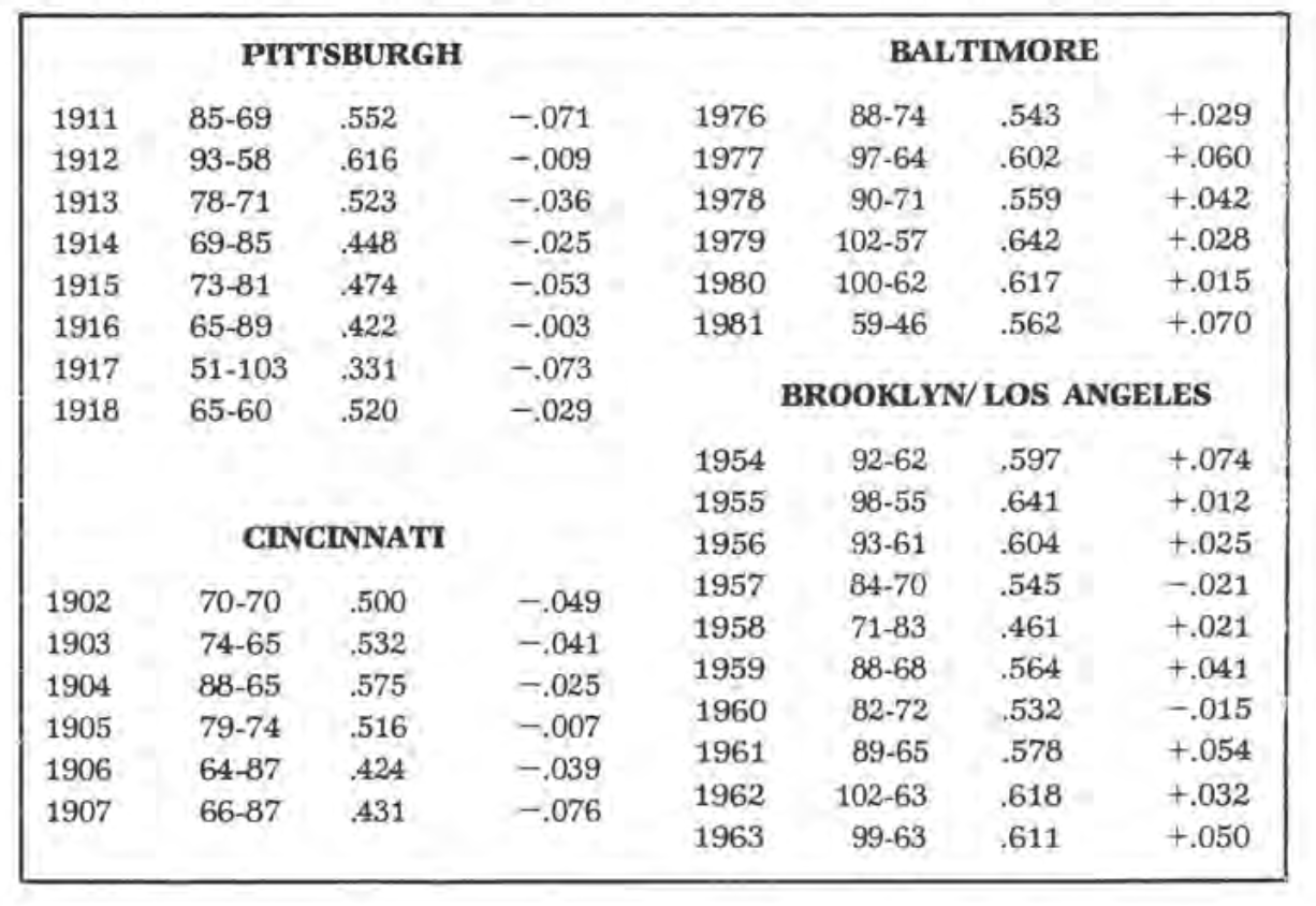
(Click image to enlarge)
PETE PALMER is chairman of SABR’s Statistical Analysis Committee.