Multi-Attribute Decision Making Ranks Baseball’s All Time Greatest Hitters

Introduction and History

I have taught or co-taught sabermetrics in the mathematics department at the United States Military Academy several times. We covered all the metrics but what always interested me most was the direction student projects took to solve or analyze various issues in baseball. In one of these courses, for example, the group project came up with a new metric for percentage of extra base hits. In reading Bill James and examining all the metrics available to enthusiastic baseball fans, it struck me that every fan has an opinion as to the best or greatest hitter ever in baseball, each using the metric that best suited their choices.

Through basic research, I found many such conclusions:

a. Ted Williams was the greatest hitter ever. 1

b. The top five hitters voted online were Ruth, Cobb, Hornsby, Gehrig, Williams. 2

c. The Britannica chose Ruth, Mays, Bonds, Williams, Aaron.3

d. Baseball’s All Time Greatest Hitters shows how statistics can level the playing field and concludes Tony Gwynn is the best.

Just Google “Greatest Hitters in Baseball All-time” and see the many results. Google found 851,000 results when I tried. Many have similar but slightly different conclusions but one thing that all seemed to have in common was their subjective nature. The basic results of (a)-(d) support that.

If raw home runs were the most important metric, the top five all time would be Barry Bonds (762), Hank Aaron (755), Babe Ruth (714), Alex Rodriguez (696), and Willie Mays (660). If hits, then Pete Rose (4256), Ty Cobb (4189), Hank Aaron (3771), Stan Musial (3630) and Tris Speaker (3514) would be the top five. Only Hank Aaron is in the top 5 in both lists. One article argues that Tony Gwynn was the all-time greatest hitter. In the table below, we present the best in the categories of home runs, extra base hits, RBIs, OBP, SLG and OP just for players who have been inducted into the National Baseball Hall of Fame in Cooperstown. It is easy to see why there are disputes.

 

Table 1. Leaders for Players in the Hall of Fame

Home Runs	Extra Base Hits	RBI	OBA	SLG	OPS
Aaron	Aaron	Aaron	Williams	Ruth	Ruth
Ruth	Musial	Ruth	Ruth	Williams	Williams
Mays	Ruth	Anson	McGraw	Gehrig	Gehrig
Griffey	Mays	Gehrig	Hamilton	Foxx	Foxx
Thome	Griffey	Musial	Gehrig	Greenberg	Greenberg

 

Table 2. Leaders for All Players

Home Runs	Extra Base Hits	RBI	OBA	SLG	OPS
Bonds	Aaron	Aaron	Williams	Ruth	Ruth
Aaron	Bonds	Ruth	Ruth	Williams	Williams
Ruth	Musial	Rodriguez	McGraw	Gehrig	Gehrig
Rodriguez	Ruth	Anson	Hamilton	Foxx	Bonds
Mays	Pujols	Pujols	Gehrig	Bonds	Foxx

 

We could perform this same exercise using newer metrics instead of counting stats, but ultimately the same debate arises. Therefore, in lieu of a single metric, I propose using a multi-attribute decision-making algorithm that allows for the use of many metrics. There is no limit to the number of metrics that might be used in such an analysis. We point out that the metrics chosen for our analysis might not be the metrics chosen by many readers.

In using multi-attribute decision-making (MADM) algorithms, the attributes (in this case the chosen baseball metrics) must have assigned weights where the sum of all weights used must equal one. The MADM algorithms themselves call for weighted metrics. Additionally, there are several weighting algorithms that can be used. Some are subjective and at least one is objective. Subjective weights are, or can be, not much different from just choosing one metric, ordering, and stating the result. However, objective weighting weights allow the data elements themselves to be used in the calculation of the weights. This appears as a more objective method as it allows the user data (as many data metrics as the user desires) to be used to calculate the weights and in a ranking decision-making algorithm. The selection of the players in the analysis, and the choice of metric used, affect the calculation of the weights and in turn the ranking of the players. We choose TOPSIS, the technique of order preference by similarity to the ideal solution, to be our MAMD algorithm because TOPSIS is the only algorithm that allows these attributes (criteria and in our case metrics) to either be selected to be maximized or minimized. For example, home runs could be maximized but perhaps strikeouts, as a metric, should be minimized.

Quantitative analysis is one method that can be used where at least the reader can see the inputs and outputs used for the analysis. The mathematics used and their results are not without fault. However, the assumptions behind the metrics and which players to use or exclude can be questioned and argued just as subjective decisions might be argued among fans. In this article, we suggest a quantitative method—the technique of order performance by similarity to ideal solution (TOPSIS)—and discuss why we think it is has merit to be used in analysis.

1. Multi-attribute Decision Making (MADM)

The two main types of multi-attribute decision methods are (1) simple additive weights (SAW) and (2) the Technique of Order Preference by Similarity to Ideal Solution (TOPSIS). These methods require a normalization process of the data and multiplication by weights found by either subjective methods or entropy. TOPSIS has a clear advantage if any of the attributes (metrics) being used should be minimized instead of maximized. As previously mentioned, home runs should be maximized but strikeouts should be minimized. If all attributes being utilized should be maximized both are adequate for analysis. But if we were using stolen bases (SB) and caught stealing (CS), then we would maximize SB and minimize CS.

The Technique of Order Preference by Similarity to Ideal Solution (TOPSIS)

TOPSIS was the result of research and work done by Ching-Lai Hwang and Kwangsun Yoon in 1981.4 TOPSIS has been used in a wide spectrum of comparisons of alternatives including: item selection from among alternatives, ranking leaders or entities, remote sensing in regions, data mining, and supply chain operations. TOPSIS is chosen over other methods because it orders the feasible alternatives according to their closeness to an ideal solution.5 Its strength over other decision making methods is that with TOPSIS, we can indicate which metric (attributes) should be maximized and which should be minimized. In all other methods, everything is maximized.

TOPSIS is used in many applications across business, industry, and government. Jeffrey Napier provided some analysis of the use of TOPSIS for the Department of Defense in industrial base planning and item selection.6 For years, the military used TOPSIS to rank order the systems’ request from all the branches within the service for the annual budget review process. MADM and TOPSIS are being taught as part of decision analysis.

So why are we using TOPSIS as our MADM method and entropy as our weighting scheme? We are using TOPSIS because in our selected dataset all variables are not “larger is better.” As mentioned, for strikeouts (SO), we’d prefer a smaller value. Entropy weights allows the data themselves to be used mathematically to calculate the weights and is not biased by subjectivity as are the other weighting schemes methods such as pairwise comparison method. Again, if we were using stolen bases (SB) in our analysis then we would like SB to be maximized and caught stealing (CS) minimized.

TOPSIS Methodology

The TOPSIS process is carried out through the following steps.

Step 1

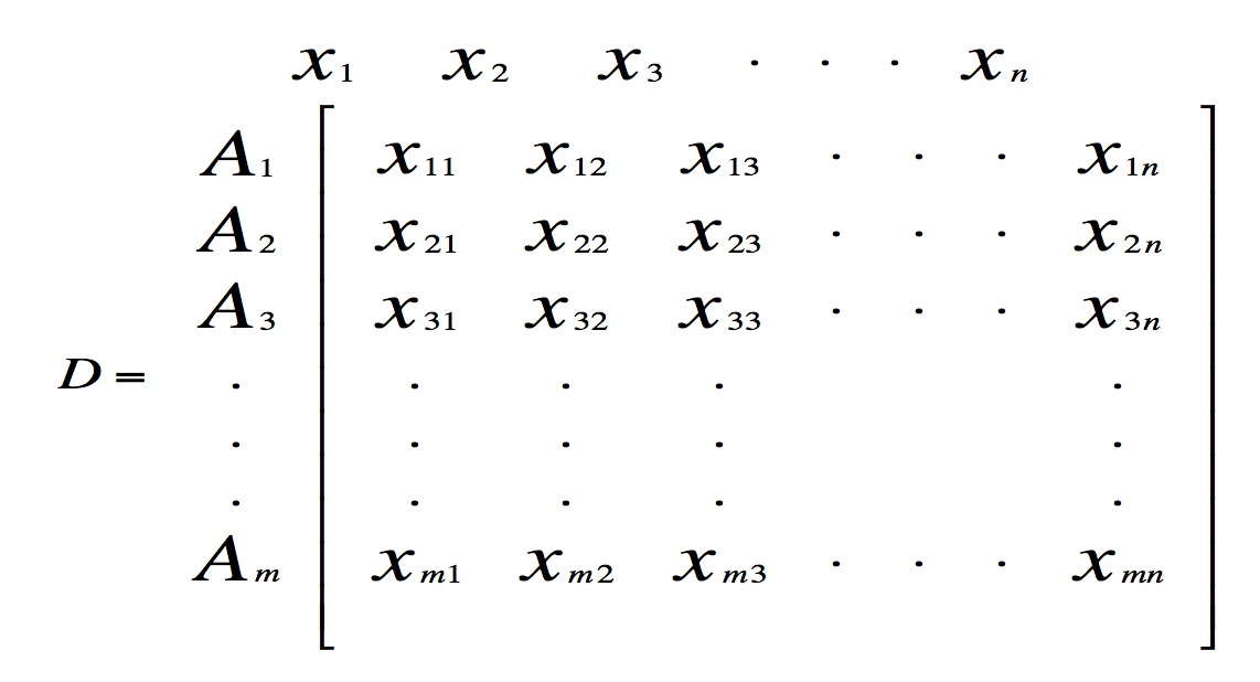
Create an evaluation matrix consisting of m alternatives (players) and n criteria (metrics), with the intersection of each alternative and criterion given as x_ij, giving us a matrix (X_ij) _mxn.

Step 2

The matrix shown as D above is then normalized to form the matrix R=(R_ij)_mxn,

using the normalization method to obtain the entries,

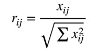
for i=1,2…,m; j= 1,2,…n

Step 3

Calculate the weighted normalized decision matrix. First, we need the weights. Weights can come from either the decision maker or by computation using entropy.

Step 3a.

Use either the decision maker’s weights for the attributes x₁,x₂,..x_n , pairwise comparisons method, or the entropy weighting scheme, as we use here.

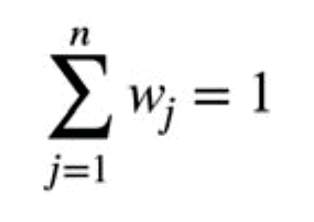
The sum of the weights over all attributes must equal one regardless of the weighting method used.

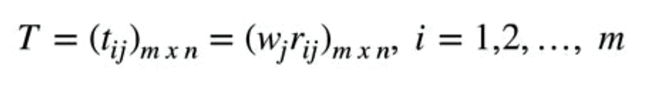
Step 3b.

Multiply the weights to each of the column entries in the matrix from Step 2 to obtain the matrix, T.

Step 4

Determine the worst alternative (A_w) and the best alternative (A_b) : Examine each attribute’s column and select the largest and smallest values appropriately. If the values imply larger is better (profit) then the best alternatives are the largest values and if the values imply smaller is better (such as cost) then the best alternative is the smallest value.

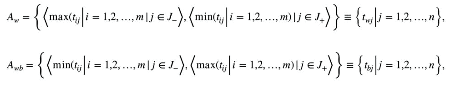
where,

J₊ = {j = 1,2,…n | j)  associated with the criteria having a positive impact, and

J_{_} = {j = 1,2,…n | j) associated with the criteria having a negative impact.

We suggest that if possible make all entry values in terms of positive impacts.

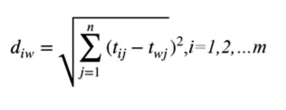
Step 5

Calculate the L2-distance between the target alternative i and the worst condition A_w

and the distance between the alternative i and the best condition A_b

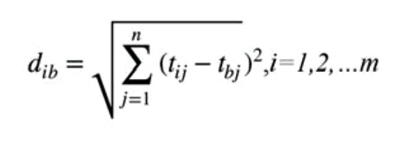
where d_iw and d_ib are L2-norm distances from the target alternative i to the worst and best conditions, respectively.

Step 6

Calculate the similarity to the worst condition:

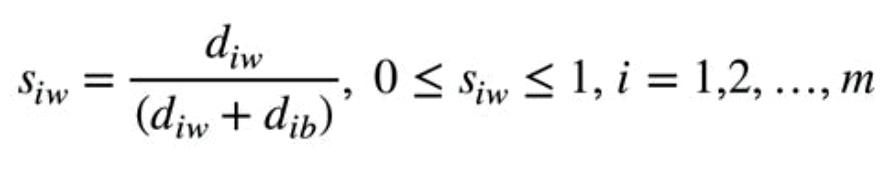
S_iw=1 if and only if the alternative solution has the worst condition; and

S_iw=0 if and only if the alternative solution has the best condition.

Step 7

Rank the alternatives according to their value from S_iw (i=1,2,…,m).

Simple Additive Weights (SAW)

SAW is a very straightforward and easily constructed process within MADM methods, also referred to as the weighted sum method.7 SAW is the simplest, and still one of the widest used of the MADM methods. Its simplistic approach makes it easy to use. Depending on the type of the relational data used, we might either want the larger average or the smaller average.

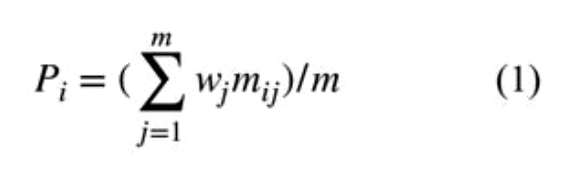
Here, each criterion (attribute) is given a weight, and the sum of all weights must be equal to one. If equally weighted criteria then we merely need to sum the alternative values. Each alternative is assessed with regard to every criterion (attribute). The overall or composite performance score of an alternative is given simply by Equation 1 with m criteria.

It was previously though that all the units in the criteria must be identical units of measure such as dollars, pounds, seconds, etc. A normalization process can make the values unitless. So, we recommend normalizing the data as shown in equation 2:

 

 

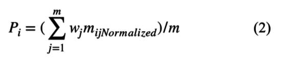
where (m_ijNormalized) represents the normalized value of m_ij, and P_i is the overall or composite score of the alternative A_i. The alternative with the highest value of P_i is considered the best alternative.

The strengths of SAW are (1) the ease of use and (2) the normalized data allow for comparison across many differing criteria. But with SAW, either larger is always better or smaller is always better. There is not the flexibility in this method to state which criterion should be larger or smaller to achieve better performance. This makes gathering useful data of the same relational value scheme (larger or smaller) essential.

Entropy Weighting Scheme

Shannon and Weaver originally proposed the entropy concept.8 This concept had been highlighted by Zeleny for deciding the weights of attributes.9 Entropy is the measure of uncertainty in the information using probability methods. It indicates that a broad distribution represents more uncertainty than does a sharply-peaked distribution. To determine the weights by the entropy method, the normalized decision matrix we call R_ij is considered. The equation used is

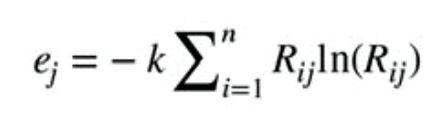
Where k = 1/ln(n) is a constant that guarantees that 0 < e_j < 1. The value of n refers to the number of alternatives. The degree of divergence (d_j) of the average information contained by each attribute is calculated as:

d_j=1-e_j.

The more divergent the performance rating R_ij, for all i & j, then the higher the corresponding d_j the more important the attribute B_j is considered to be.

The weights are found by the equation,

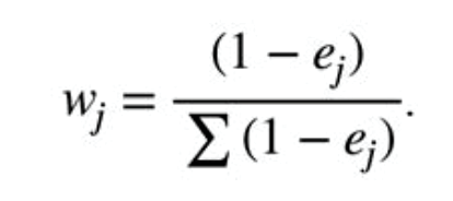
Let’s assume that the criteria were listed in order of importance by a decision maker. Entropy ignores that fact and uses the actual data to compute the weights. Although home runs might be the most important criterion to the decision maker, it might not be the largest weighted criterion using entropy. Using this method, we must be willing to accept these types of results in weights.

Sensitivity Analysis

In the previous work done by Fox and Fox et al. using the pairwise comparison method of obtaining weight, sensitivity analysis was done to determine the effect of changing weights on the ranking of terrorists.10 The decision weights are subject to sensitivity analysis to determine how the affect the final ranking. Sensitivity analysis is essential to good analysis. Additionally, Alinezhad suggests sensitivity analysis for TOPSIS for changing an attribute weight.11 The equation they developed for adjusting weights based upon a single weight change that we used is:

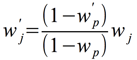
where w_j’ is the future weight of criterion j, w_p the current selected weight to be changed, w_p’ the new value of the selected weight, wj is the current weight of criterion j. This method of doing sensitivity analysis is valid for any chosen weighting scheme.

Another method of sensitivity analysis might be to change the metric used or the baseball players used in the analysis. We accomplished this by first including strikeouts and then excluding strikeouts in our analysis. We also can alter the players used if we are using the entropy weighting methods. Changing players, as well as changing metrics analyzed, changes the weights that are calculated and in turn might change the rank ordering of the players.

Application to Baseball’s Greatest Hitters

We applied these mathematical techniques to baseball’s greatest hitters. We started by taking hitters in the National Baseball Hall of Fame (excluding pitchers and managers). We ran our analysis. Then we added some star retired players and current players: Pete Rose, Barry Bonds, Mark McGwire, Alex Rodriguez, Albert Pujols, Mike Trout, Miguel Cabrera, Sammy Sosa, and Ichiro Suzuki, sourcing their statistics from Baseball-Reference.com.12,13

Data

Based upon reviewers’ comments, we ran several separate analyses with the Hall of Fame players as well as the Hall of Famers including the additional mentioned players. We used standard metrics as the criteria for the initial analysis and then more advanced metrics for the second run of our analysis. 14

Standard Metrics

• G: Games Played
• PA: Plate Appearances
• AB: At Bats
• R: Runs Scored
• H: Hits
• 2B: Doubles Hit
• 3B: Triples Hit
• HR: Home Runs Hit
• RBI: Runs Batted In
• BB: Bases on Balls
• SO: Strikeouts
• BA: Hits/At Bats

Advanced Metrics

• OBA: (H + BB + HBP)/(At Bats + BB + HBP + SF)
• SLG: Total Bases/At Bats or (1B + 2*2B + 3*3B + 4*HR)/AB
• OPS: On-Base + Slugging Averages

In our first analysis, we used the first 11 metrics above. In our second analysis we decided to use percentage of extra base hits (2B+3B+HR/hits), runs, BB, OBA and SLG. Since OPS is the sum of OBA and SLG, we excluded it from either analysis.

Since entropy is a function of the data, we separated our collected data into sets both with only the data partitioned as stated and for our two separate groups of players. First, we performed our analysis for the Hall of Fame players and then we repeat it for these same players but with the additional players added. We used the entropy method to weigh these criteria for the analysis. We did so because we did not want bias to interfere with our weighting scheme as the other methods for obtaining weights are very subjective. Using the entropy weighting scheme as described in section 2.2, we found our weights to use in the analysis. Examining the Hall of Fame set, we used the entropy method of weighting for the 11 criteria. We found these weights for the Hall of Fame players:

 

G	0.04128
PA	0.05064
AB	0.04965
R	0.06426
H	0.05876
2B	0.07295
3B	0.11743
HR	0.23904
RBI	0.07459
BB	0.09882
SO	0.12679
BA	0.00579

 

We found the weights for the second set of metrics for the Hall of Fame players as:

 

%X	RBI	BB	BA	OBA	SLG
0.149467087	0.295852	0.465290109	0.016695	0.01822	0.054477

 

We present the weights when all our additional players are included with the Hall of Fame players in the analysis.

 

Larger metric set

G	0.04847
AB	0.04886
R	0.05541
H	0.05014
2B	0.05764
3B	0.06165
HR	0.41781
RBI	0.05905
BB	0.08292
SO	0.08865
BA	0.02941

 

Smaller metric set

%X	RBI	BB	BA	OBP	SLG
0.155603773	0.292877	0.463543085	0.015732	0.017507	0.054736

 

MADM Model Results

Using our TOPSIS procedures and using “larger is better” for all variables except SO where smaller is better, we found the top Hall of Fame hitters of all time. TOPSIS ranked them in order as: Babe Ruth, Hank Aaron, Willie Mays, Stan Musial, and Lou Gehrig using our larger group of metrics.

 

Player	TOPSIS Value	Rank
Babe Ruth	0.731603653	1
Hank Aaron	0.712828581	2
Willie Mays	0.688321995	3
Stan Musial	0.664775607	4
Lou Gehrig	0.653080437	5
Ted Williams	0.639868853	6
Jimmie Foxx	0.623135348	7
Mel Ott	0.619731627	8
Frank Robinson	0.616727014	9
Ken Griffey Jr.	0.602640058	10
Ernie Banks	0.573236285	11
Mickey Mantle	0.572825146	12
Harmon Killebrew	0.566824198	13
Eddie Mathews	0.565000206	14
Frank Thomas	0.561931931	15
Mike Schmidt	0.559451492	16
Carl Yastrzemski	0.556948693	17
Eddie Murray	0.555682669	18
Willie McCovey	0.552158735	19
Dave Winfield	0.536912893	20

 

The next twenty are:

Billy Williams	0.535553305	21
Joe DiMaggio	0.534463121	22
Al Kaline	0.526047568	23
Reggie Jackson	0.523830476	24
Cal Ripken	0.520103131	25
Andre Dawson	0.508935302	26
Jeff Bagwell	0.506944011	27
Rogers Hornsby	0.506190846	28
Johnny Mize	0.503463982	29
George Brett	0.499767024	30
Duke Snider	0.497691125	31
Yogi Berra	0.495176578	32
Willie Stargell	0.493824724	33
Al Simmons	0.490040488	34
Mike Piazza	0.483583075	35
Goose Goslin	0.474848669	36
Ralph Kiner	0.473649418	37
Ty Cobb	0.46631062	38
Jim Rice	0.460974189	39
Johnny Bench	0.459232829	40

 

When we ran the analysis with the second criteria using the MADM method, SAW, because all the metrics used were to be maximized. We found that our top players were:

 

Player

Babe Ruth

Ted Williams

Lou Gehrig

Jimmie Foxx

Hank Greenberg

Mickey Mantle

Stan Musial

Joe DiMaggio

Frank Thomas

 

Note that number one in both approaches among the Hall of Fame players is Babe Ruth.

“What if” Analysis: Other non-HOF Players Included

Next, we included additional players based upon their performance, and not regarding other issues. We included Pete Rose, Barry Bonds, Mark McGwire, Alex Rodriguez, Albert Pujols, Miguel Cabrera, Mike Trout, Sammy Sosa and Ichiro Suzuki. First, we re-compute the entropy weights and then our ranking.

We present the top 20 ranked players using TOPSIS using all the chosen metrics.

The addition of the new players yielded a slightly different set of results but we see Ruth and Aaron are ranked one and two:

Babe Ruth	0.72214	1
Hank Aaron	0.70117	2
Barry Bonds	0.69878	3
Willie Mays	0.67513	4
Stan Musial	0.6537	5
Lou Gehrig	0.64057	6
Ted Williams	0.63168	7
Jimmie Foxx	0.61065	8
Mel Ott	0.61013	9
Frank Robinson	0.60508	10
Ken Griffey	0.59135	11
Alex Rodriguez	0.58904	12
Mickey Mantle	0.56287	13
Ernie Banks	0.5604	14
Harmon Killebrew	0.55695	15
Eddie Mathews	0.55434	16
Frank Thomas	0.55274	17
Carl Yastrzemski	0.54894	18
Mike Schmidt	0.54886	19
Mark McGwire	0.54863	20

 

We also ran analysis with a smaller number of metrics as mentioned earlier. The Top 25 of all time, including our stars that are not currently in the Hall of Fame, are:

 

Barry Bonds	1
Babe Ruth	2
Hank Aaron	3
Alex Rodriguez	4
Willie Mays	5
Albert Pujols	6
Ken Griffey Jr.	7
Frank Robinson	8
Sammy Sosa	9
Reggie Jackson	10
Jimmie Foxx	11
Ted Williams	12
Harmon Killebrew	13
Mike Schmidt	14
Mickey Mantle	15
Stan Musial	16
Mel Ott	17
Mark McGwire	18
Lou Gehrig	19
Frank Thomas	20
Eddie Murray	21
Eddie Mathews	22
Willie McCovey	23
Carl Yastrzemski	24
Ernie Banks	25

 

We see that using the smaller list of metrics Barry Bonds computes as first followed by Babe Ruth. The addition of the new players has made a difference in the ranking of baseball’s greatest hitters.

Conclusions

Using entropy as our method to obtain weights, which is an unbiased weighting method, we found Babe Ruth as the greatest hitter in many of our analyses, while Barry Bonds ranked number one using the smaller metric set. Arguments can be made for any of these players being the greatest hitter of all time. By using more than one sabermetric measure, applying weights to the metrics, and applying a MADM method, we can strengthen the argument for the greatest hitter of all time. Depending on the players and metrics in the analysis, we see that ranking might change. This is why the argument continues regarding who is the greatest hitter of all time?

WILLIAM P. FOX is an Emeritus professor at the Naval Postgraduate School in Monterey, CA. He is currently an adjunct professor of mathematics at the College of William and Mary in Williamsburg, VA, where he teach applied mathematics courses. He has authored over twenty books, over twenty additional chapters in other books and over a hundred journal articles.

 

Acknowledgments

I acknowledge and thank Father Gabe Costa, Department of Mathematical Sciences, United States Military Academy for introducing me to sabermetrics and the initial reading and suggestions on this research.

 

Notes

1 Tim Kurkjian, Obituary of Ted Williams, July 5, 2002, ESPN.com, accessed September 2017. http://www.espn.com/classic/obit/williams_ted_kurkjian.html

2 Ranker.com, “Best Hitters in Baseball History,” crowdranked list, accessed January 2019. http://www.ranker.com/crowdranked-list/best-hitters-in-baseball-history,

3 Britannica.com, “10 Greatest Baseball Players of All Time,” accessed January 2019. http://www.britannica.com/list/10-greatest-baseball-players-of-all-time

4 Ching-Lai Hwang and Kwangsun Yoon, 1981. Multiple attribute decision making: Methods and applications. New York: Springer-Verlag.

5 Jacek Malczewski, “GIS-Based Approach to Multiple Criteria Group Decision-Making.” International Journal of Geographical Information Science – GIS , 10(8), 1996, 955-971.

6 Jeffrey Napier. 1992. Industrial base program item selection indicators analytical enhancements. Department of Defense Pamphlet, DLA-93-P20047.

7 P.C. Fishburn (1967). Additive utilities with incomplete product set: Applications to
priorities and assignments. Operations Research Society of America (ORSA), 15, 537-542

8 Claude Shannon and Warren Weaver. 1949. The Mathematical Theory of Communication, University of Illinois Press.

9 Milan Zeleny. 1982. Multiple Criteria Decision Making. New York: McGraw Hill.

10 William Fox, Bradley Greaver, Leo Raabe, and Rob Burks. 2017. “CARVER 2.0: Integrating Multi-attribute Decision Making with AHP in Center of Gravity Vulnerability Analysis,” Journal of Defense Modeling and Simulation, Published online first, http://journals.sagepub.com/doi/abs/10.1177/1548512917717054

11 Alireza Alinezhad and Abbas Amini, 2011. “Sensitivity Analysis of TOPSIS technique: The results of change in the weight of one attribute on the final ranking of alternatives.” Journal of Optimization in Industrial Engineering, 7(2011), 23-28.

12 Hall of Fame Players Baseball Statistics, https://www.baseball-reference.com/awards/hof_batting.shtml, accessed September 14, 2017.

13 Player statistics pages from Baseball-Reference.com, Mike Trout, Pete Rose, Barry Bonds, Mark McGwire, Alex Rodriguez, Joe Jackson, Albert Pujols, Miguel Cabrera, Ichiro Suzuki, Sammy Sosa.

14 Hall of Fame Batting, https://www.baseball-reference.com/awards/hof_batting.shtml, accessed October 1, 2019.